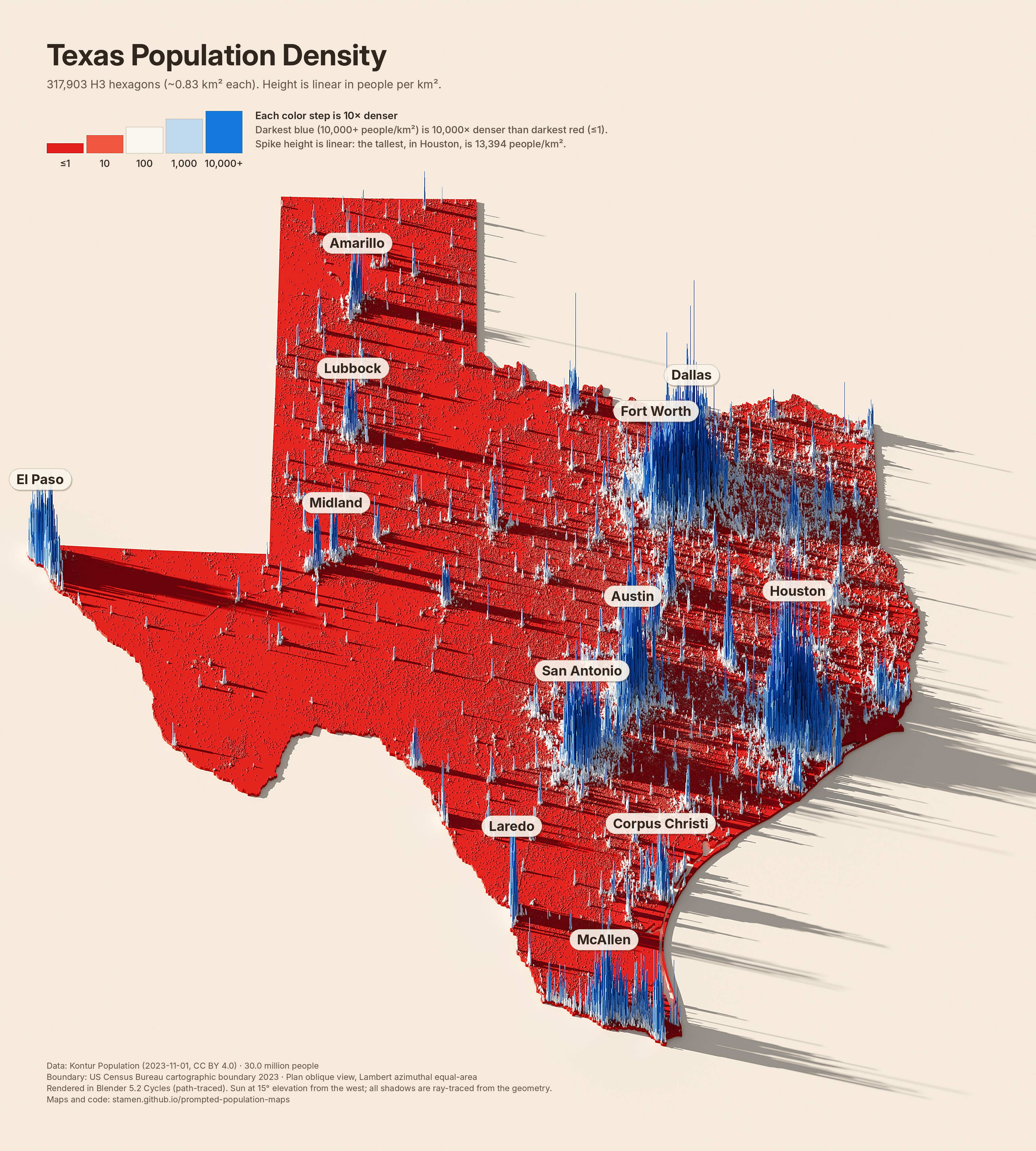
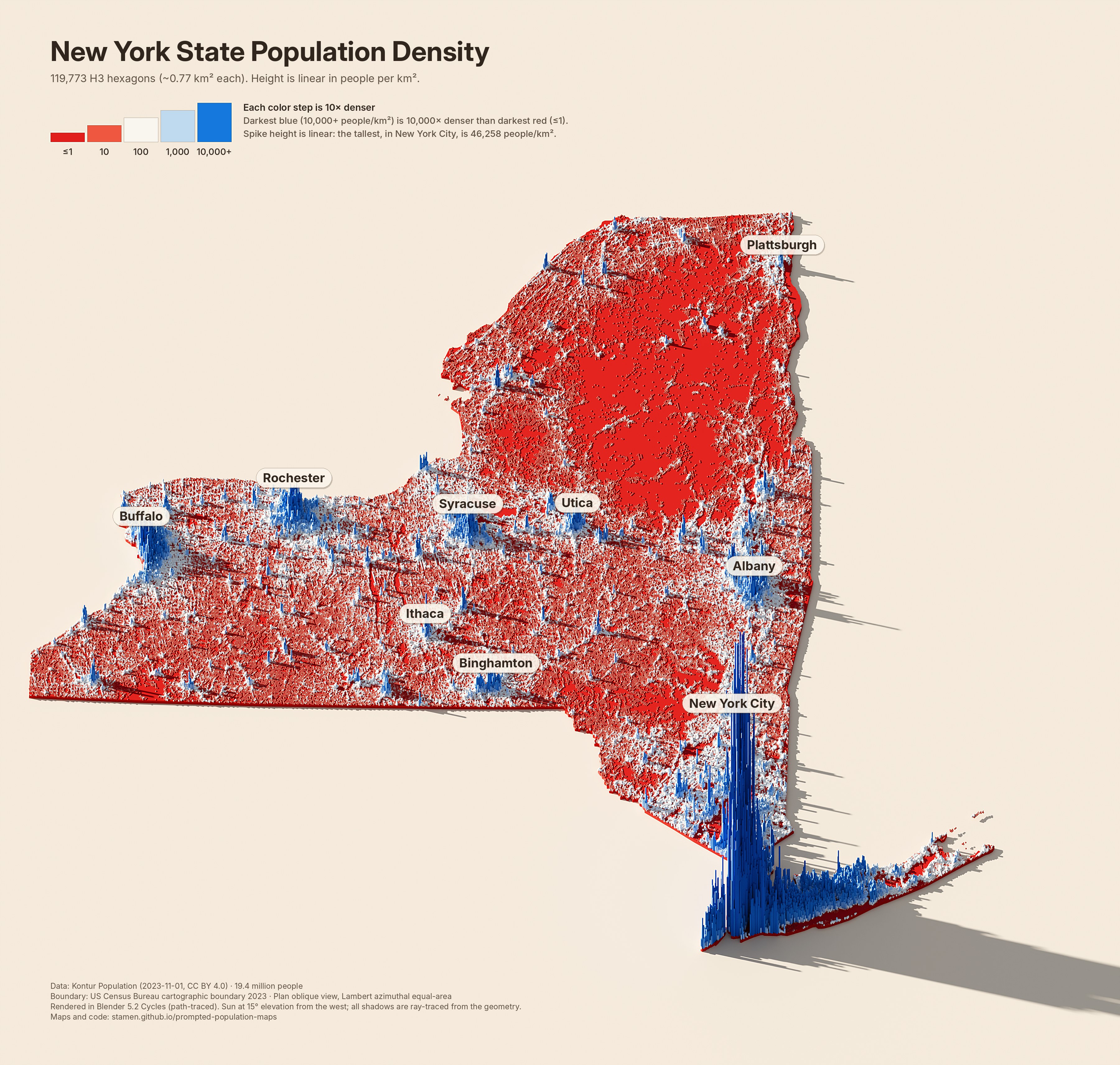
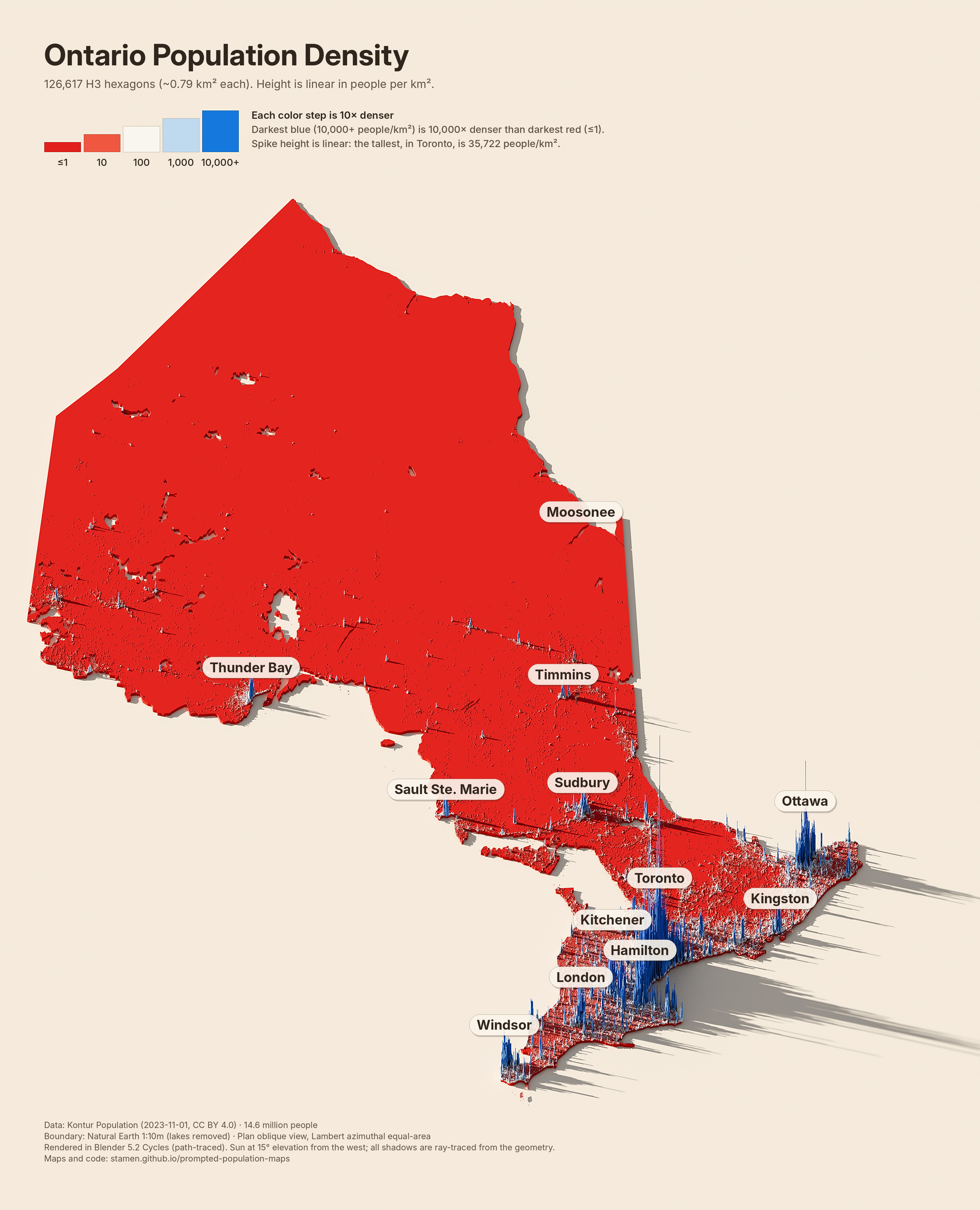
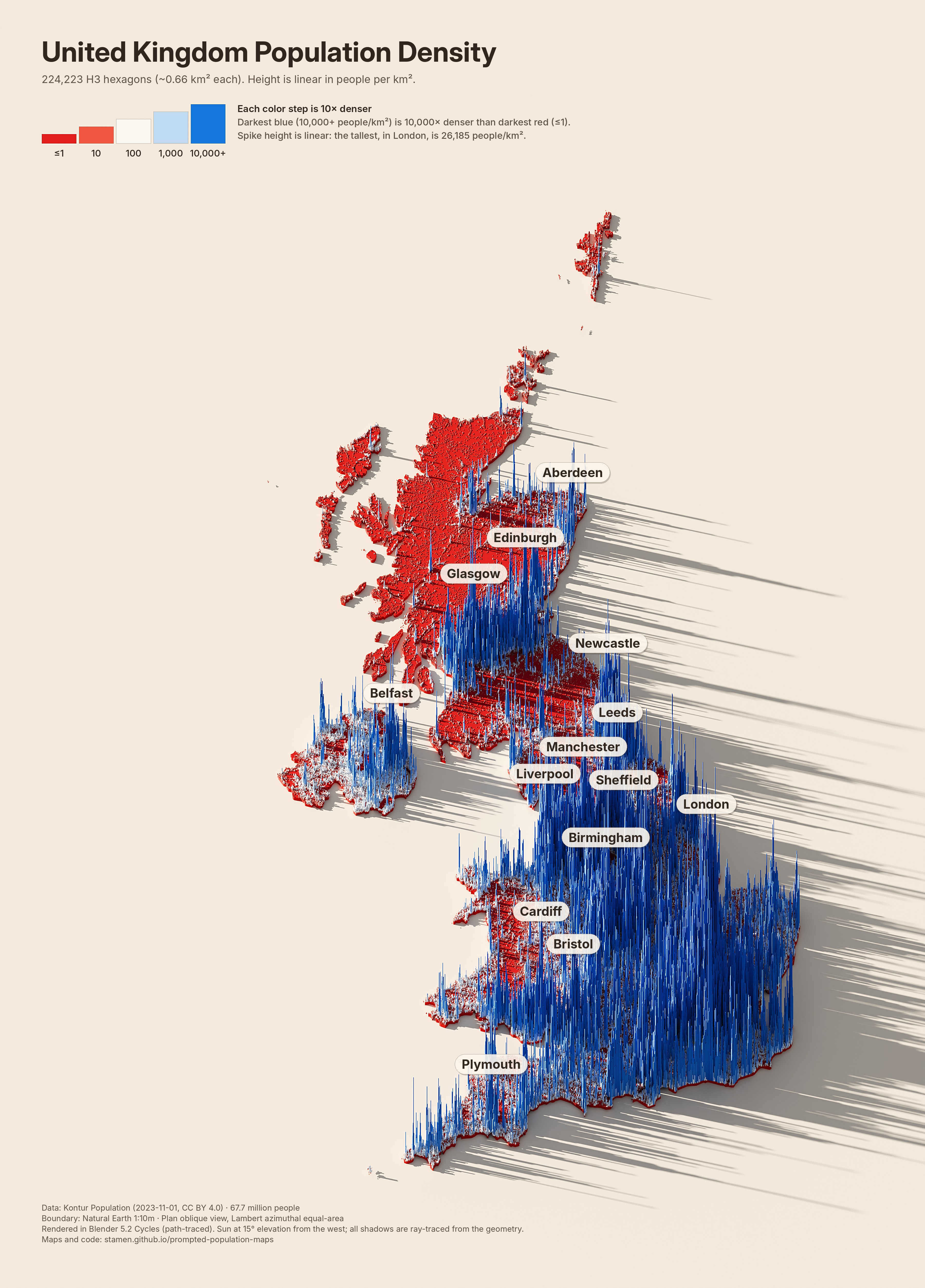
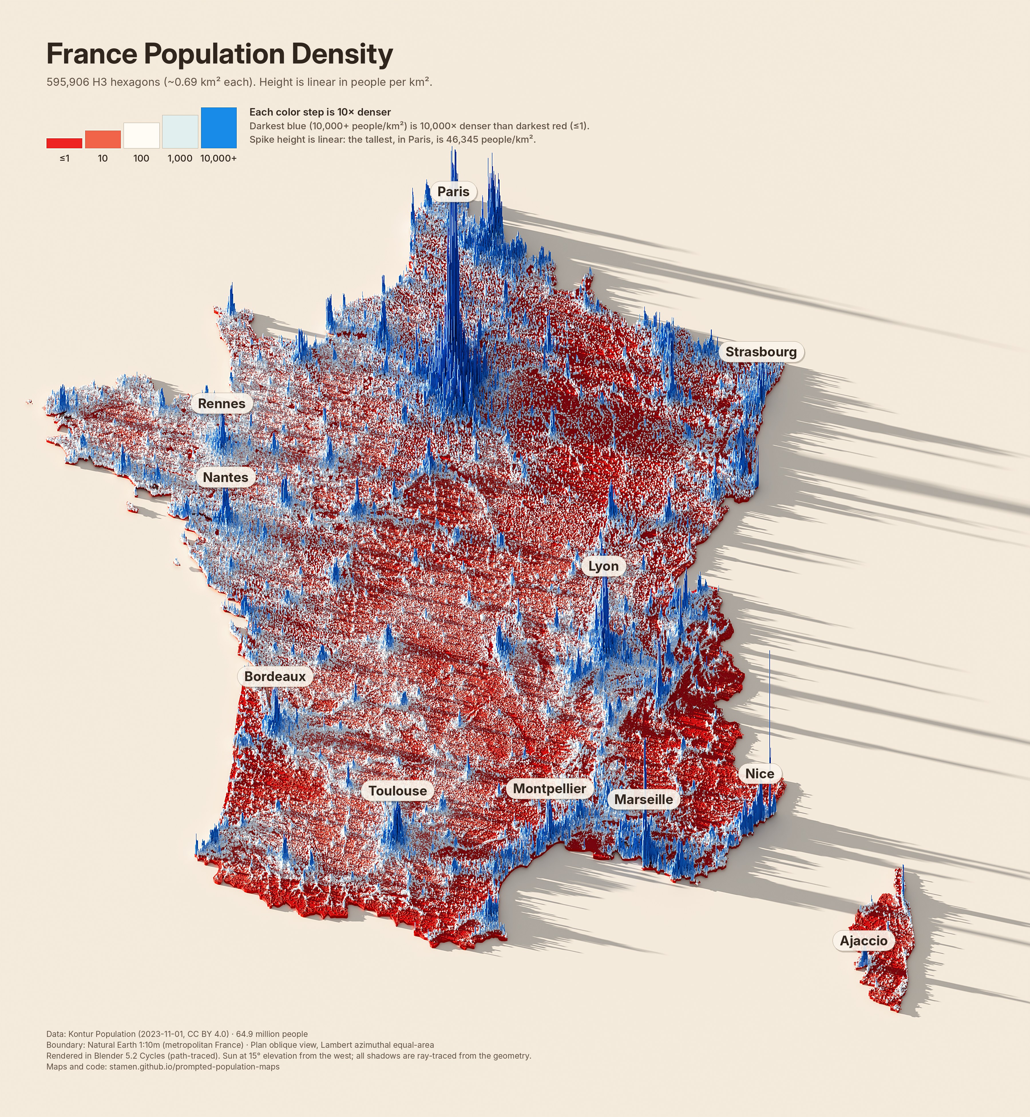
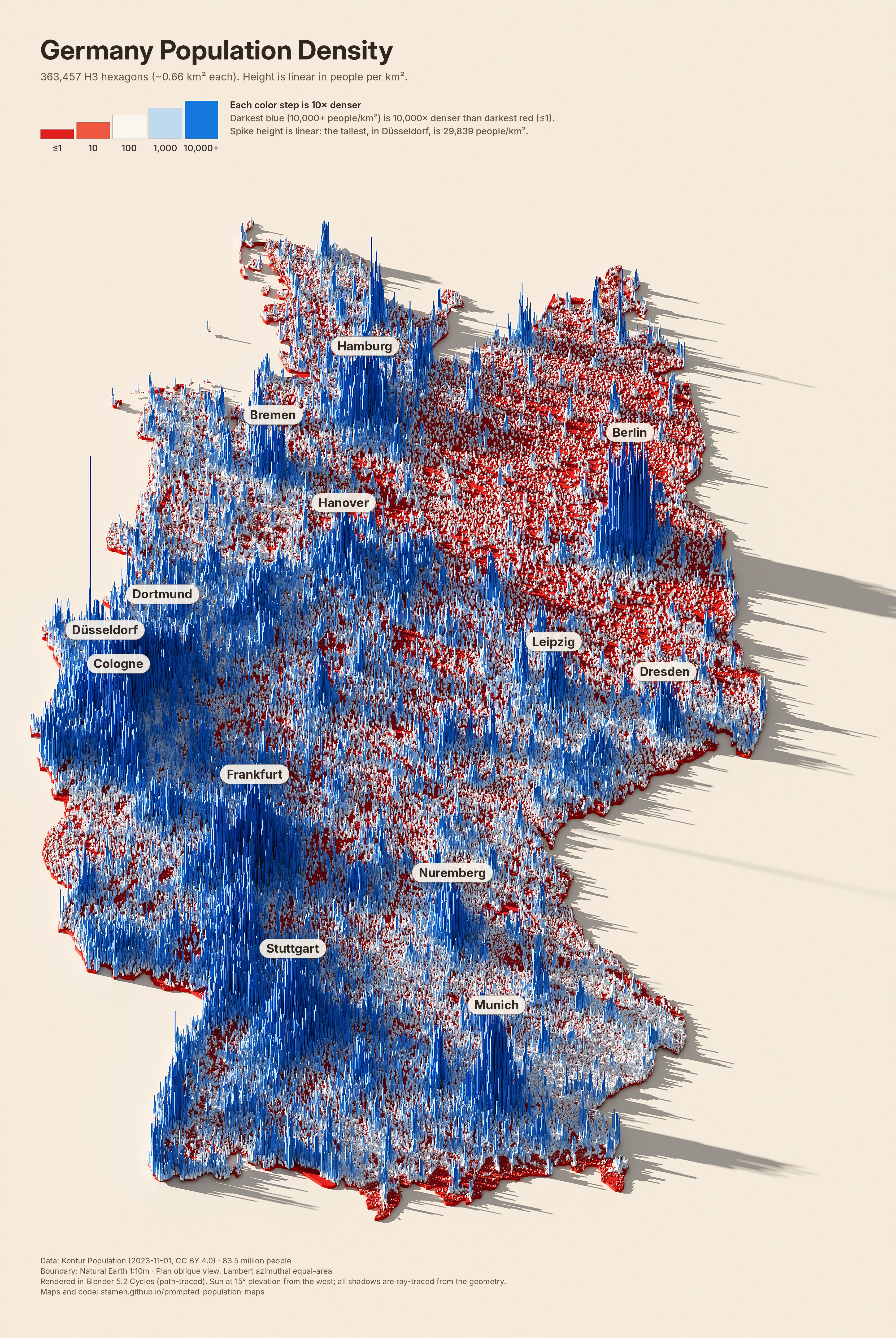
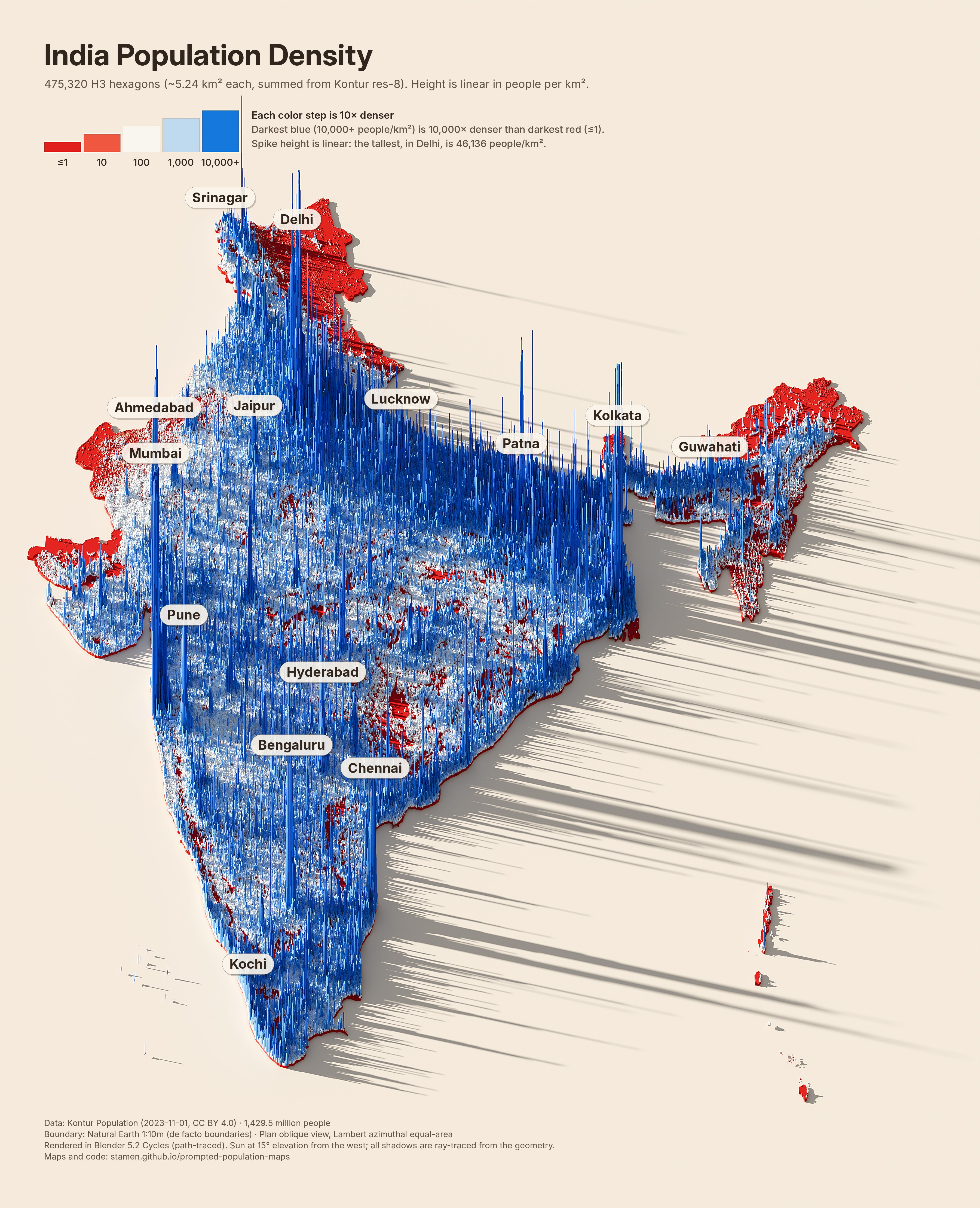
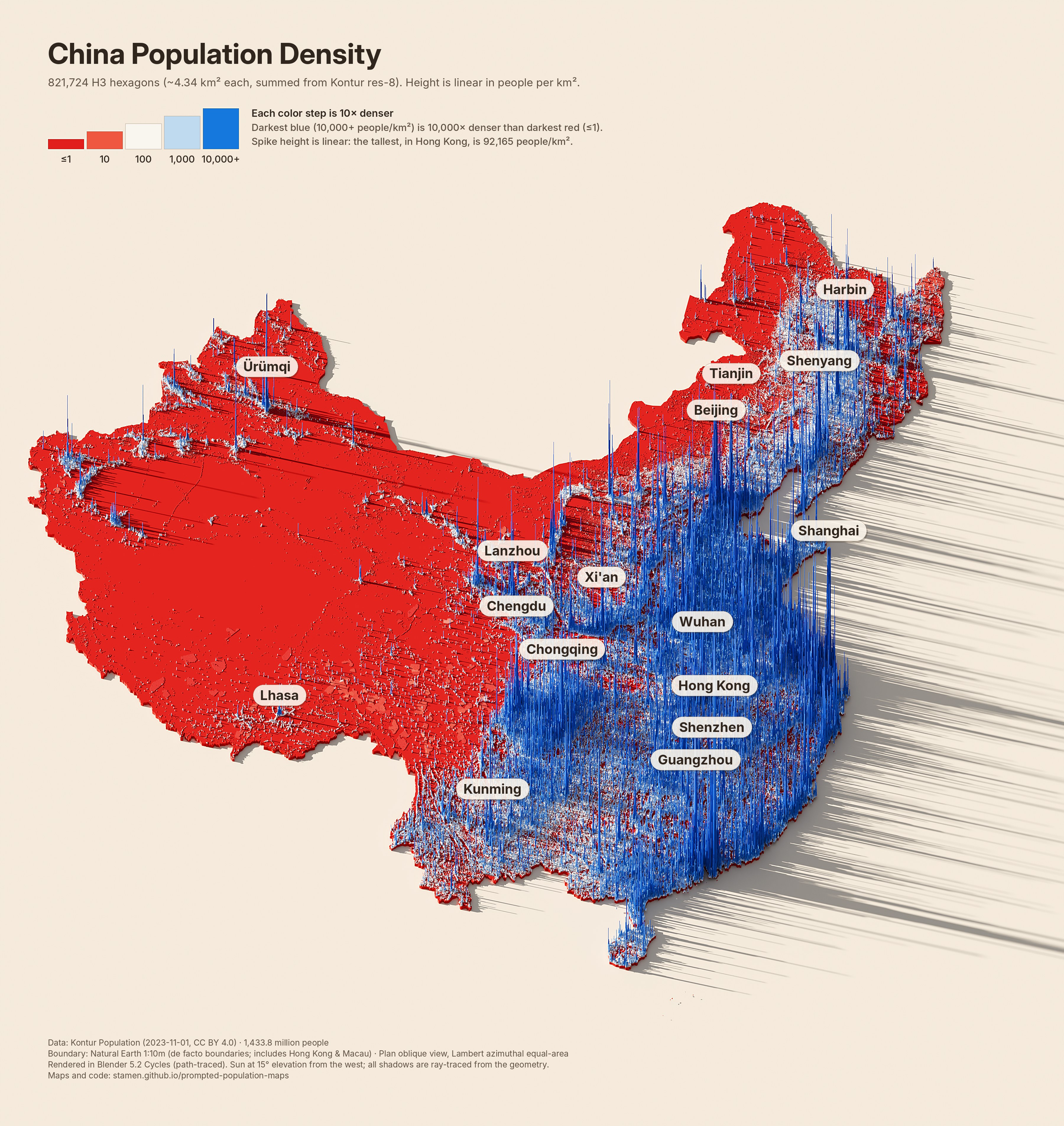
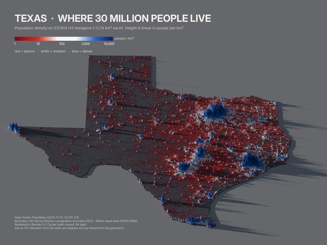
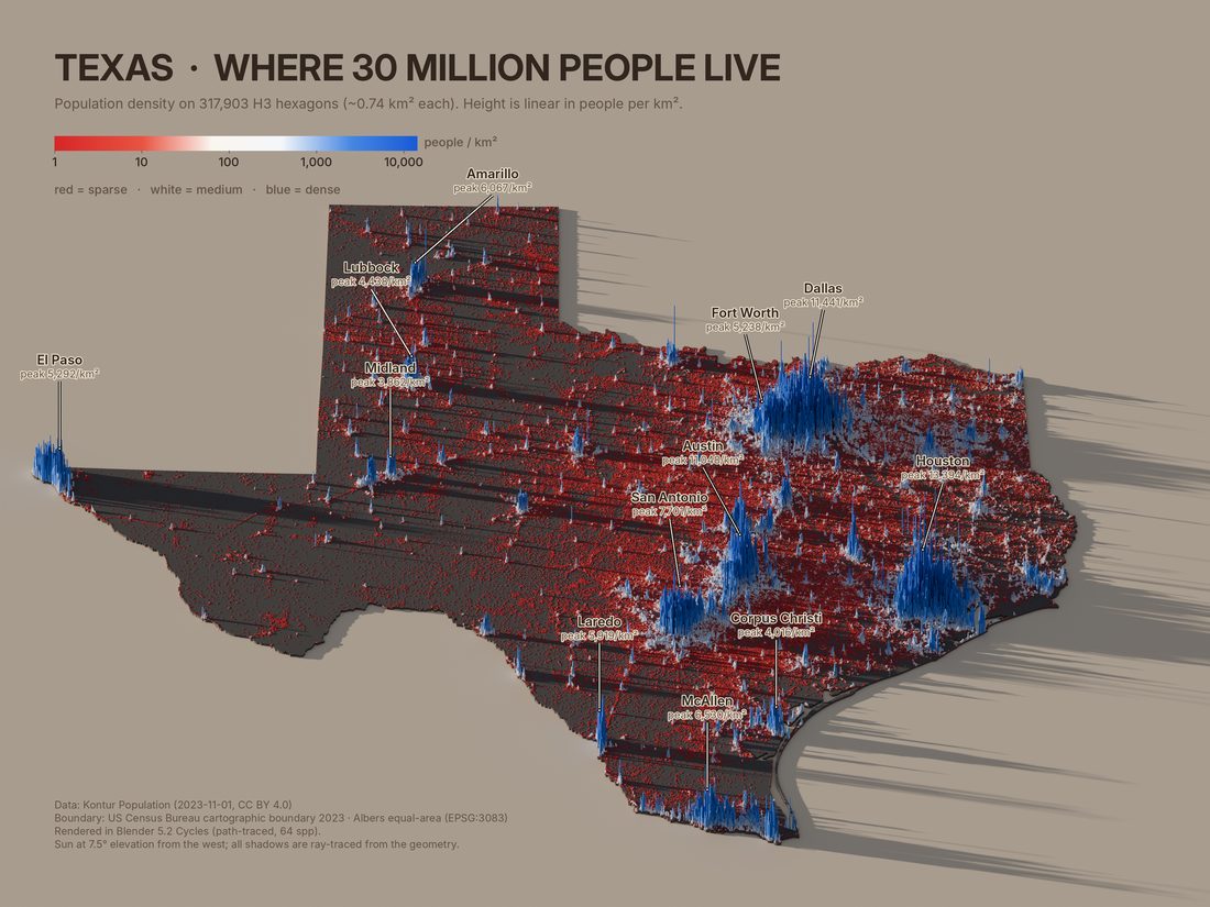
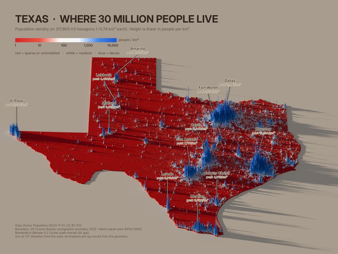
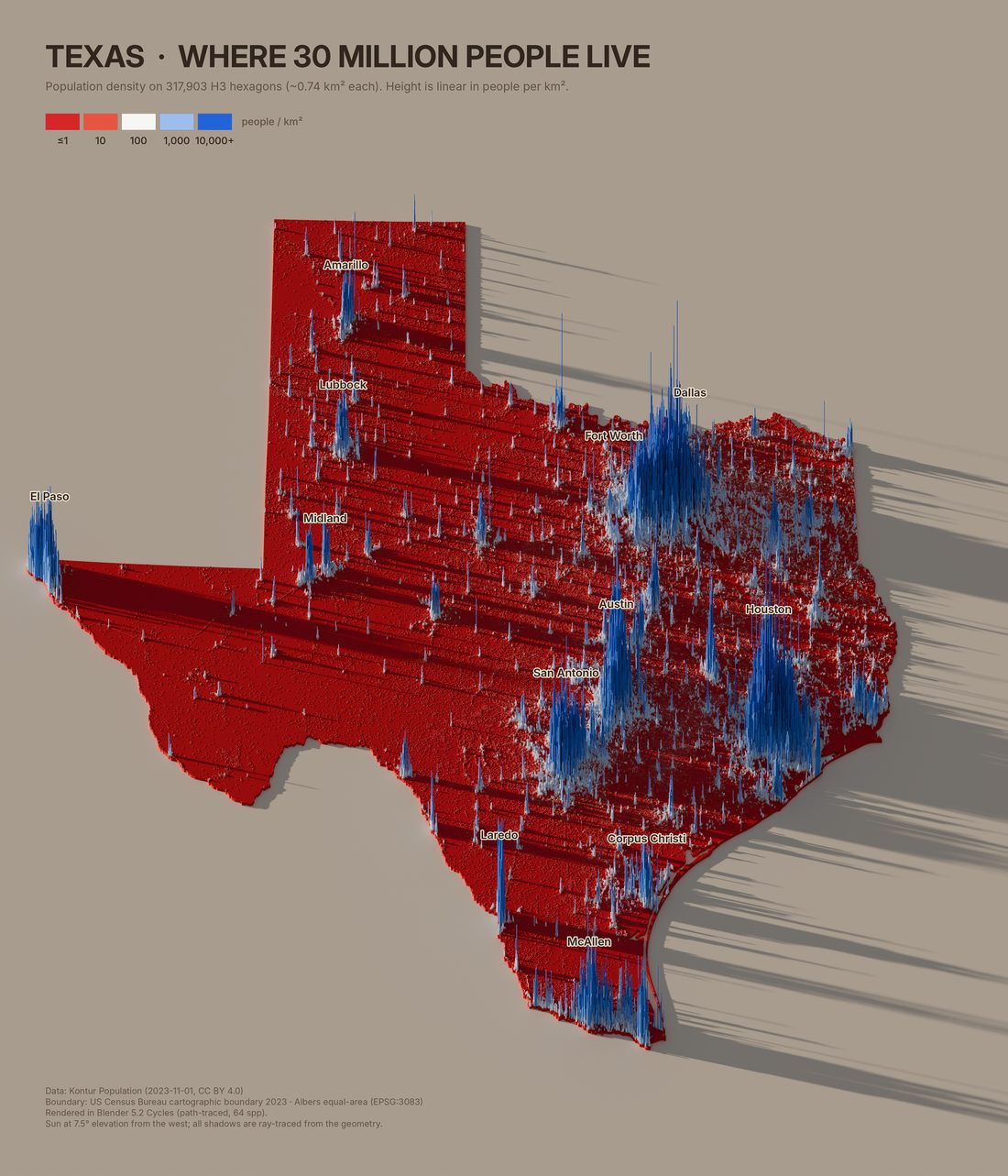
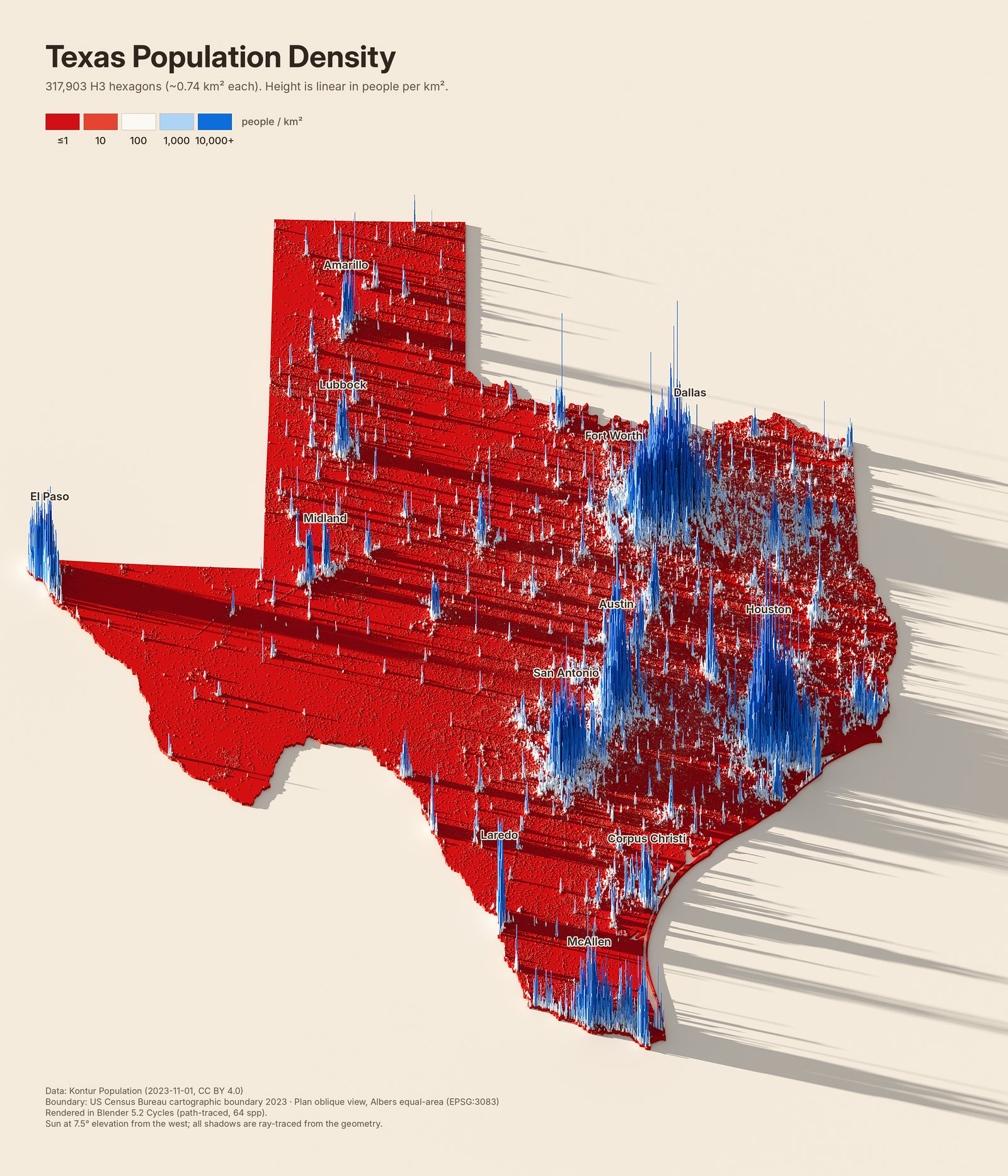
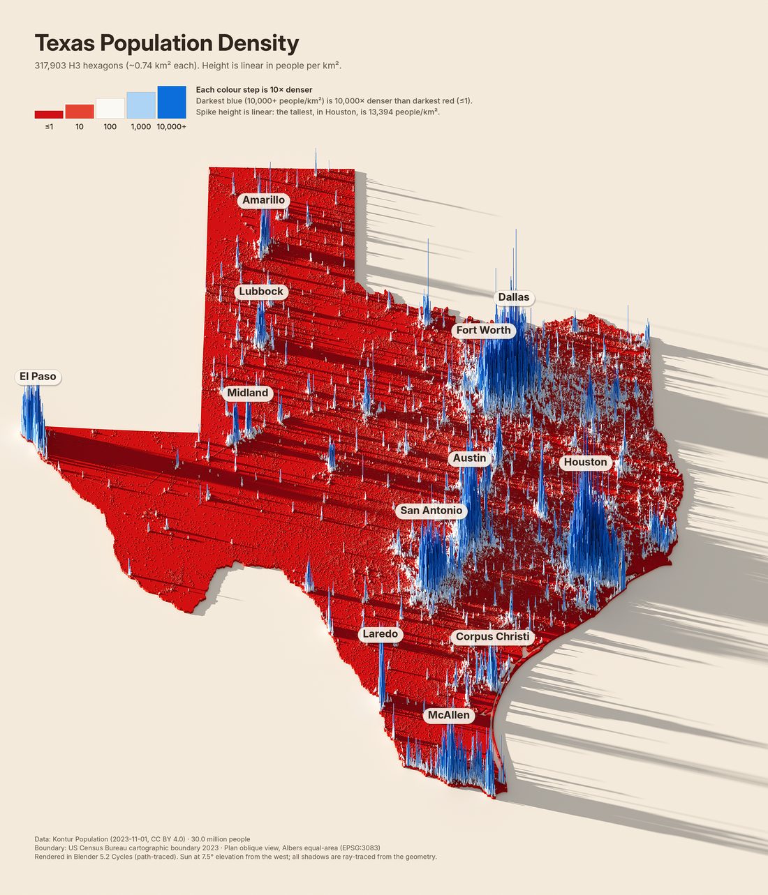
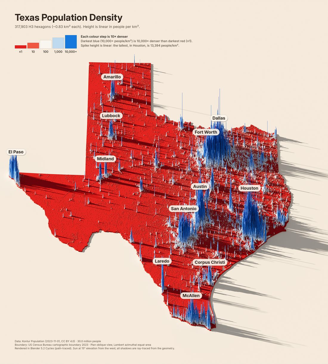
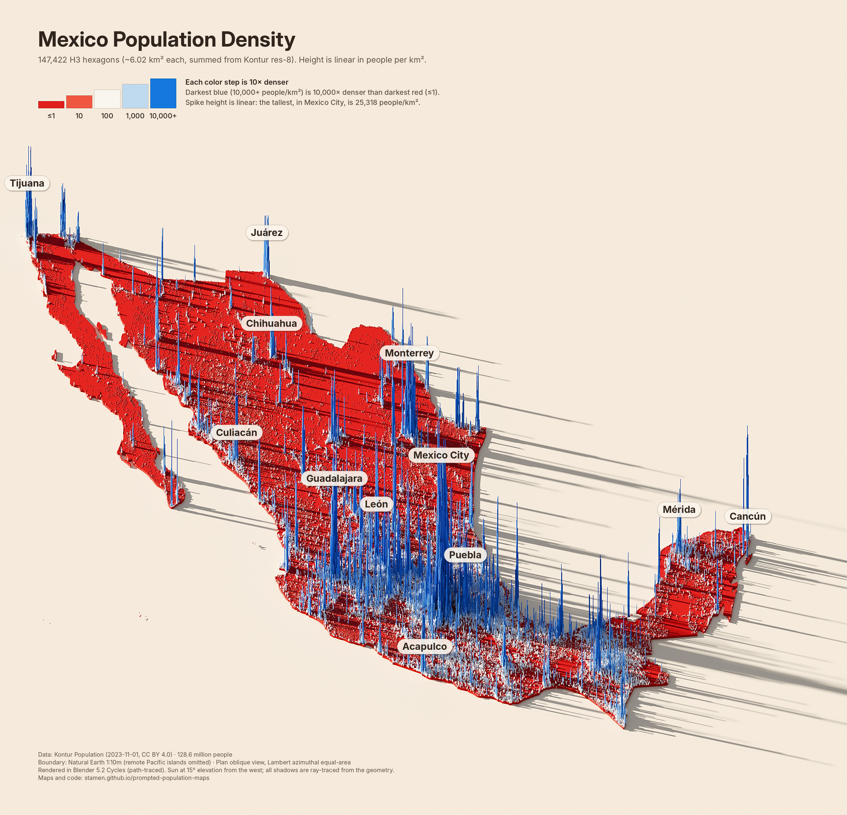
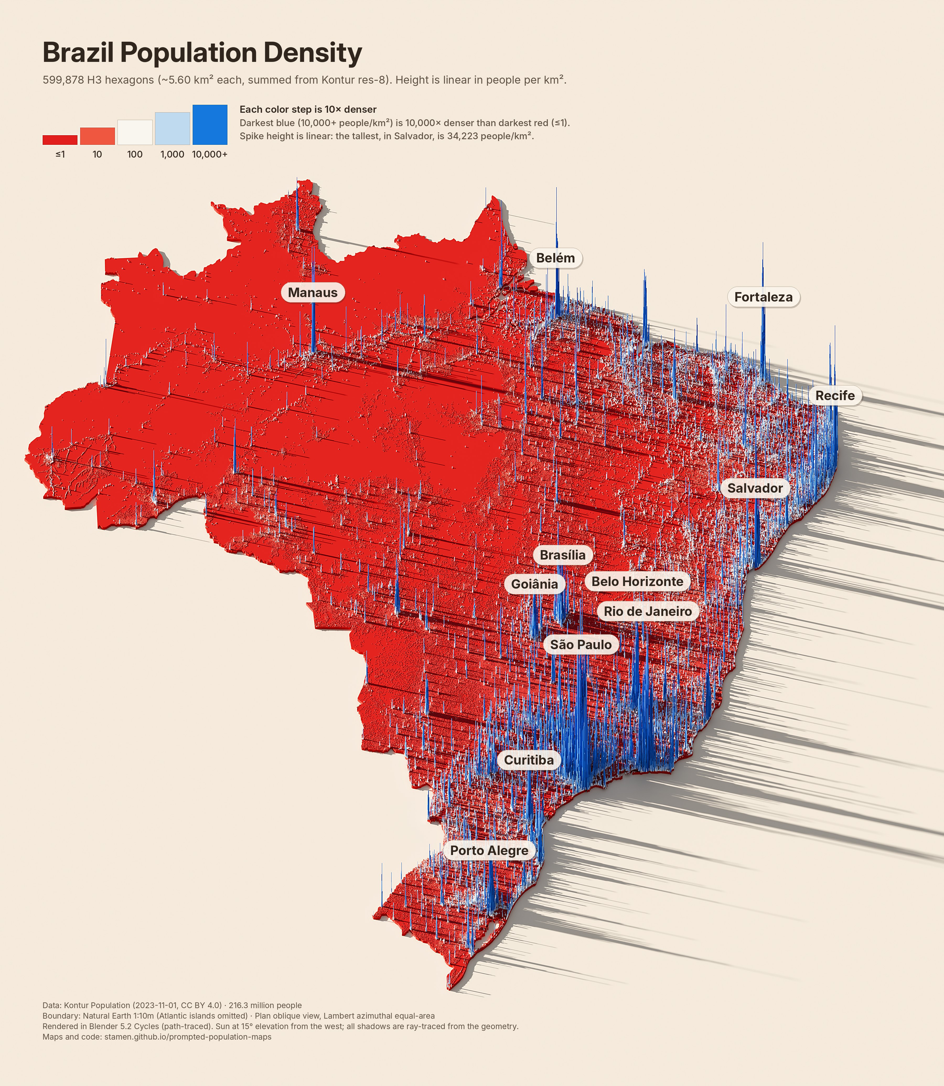
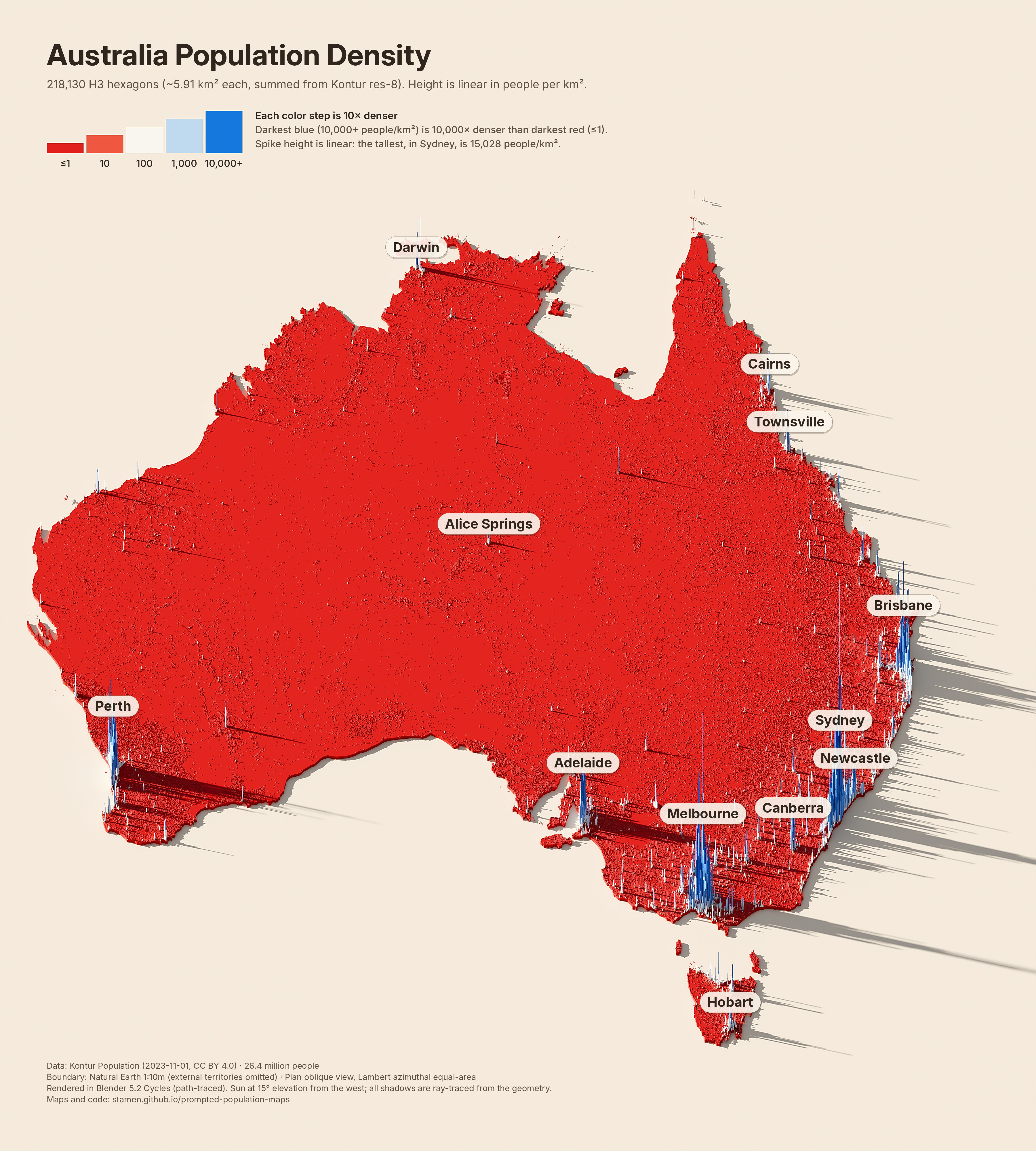
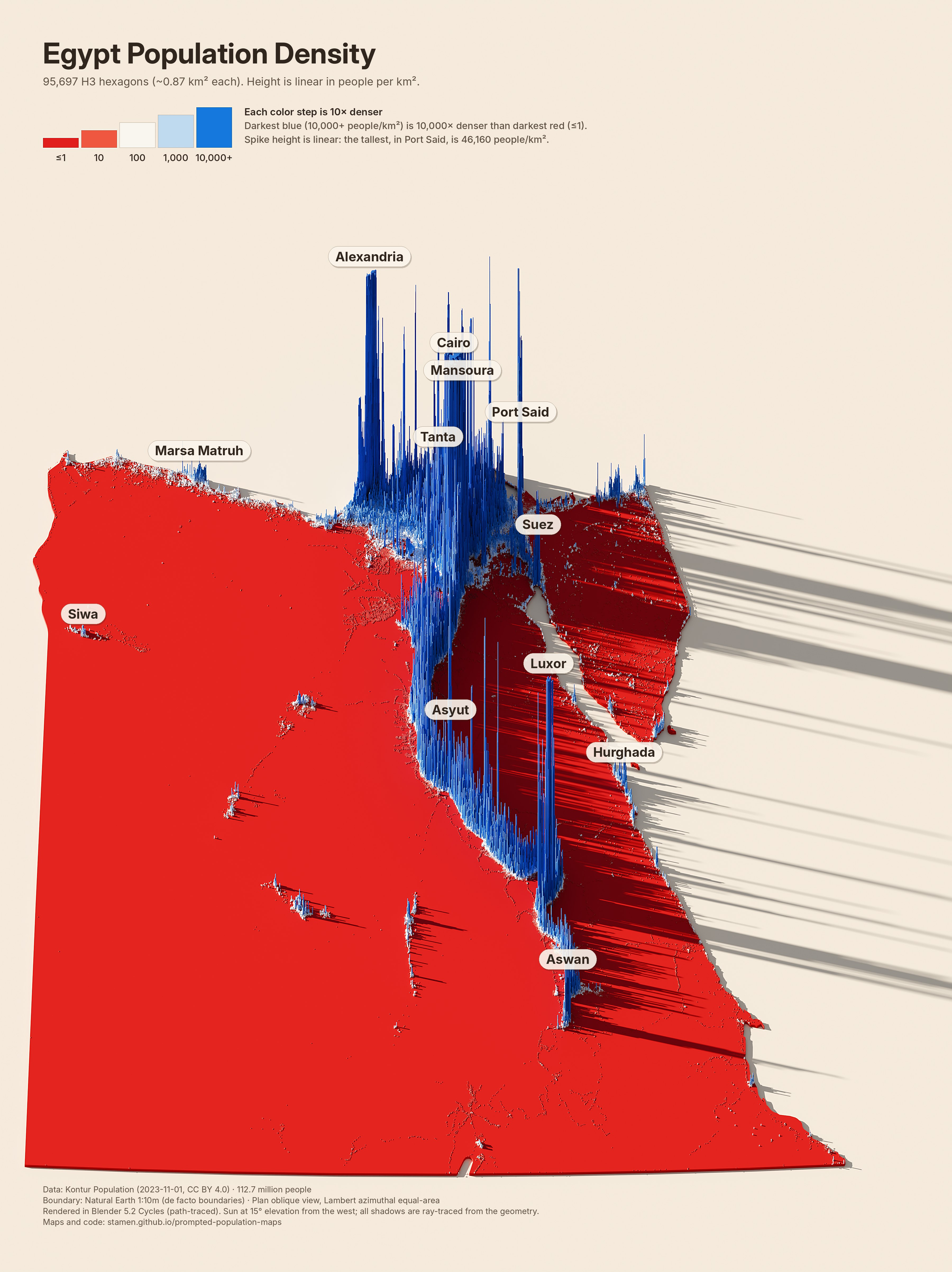
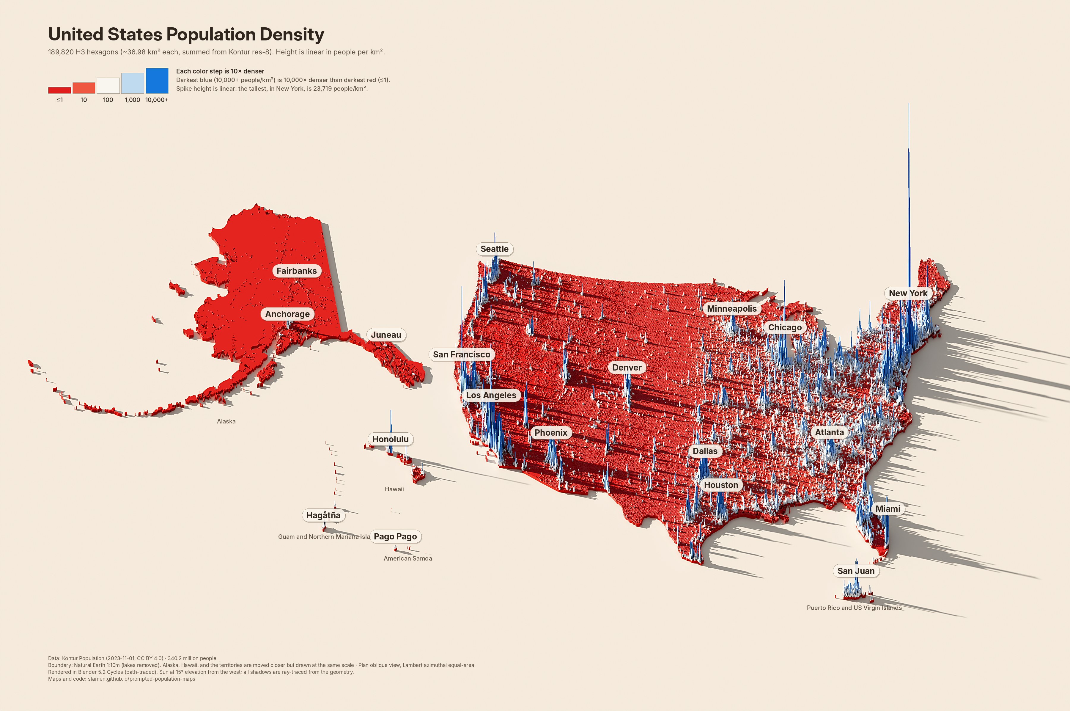
Raytraced population density maps where every inhabited H3 hexagon is extruded by its people per km², then path-traced under a low western sun. The heights come straight from the data, and every shadow is cast by the real geometry.
Several years ago I wrote a blog post called “Shadows on maps are getting a lot more exciting, and here’s why,” exploring this style of cartography, which I called “Blender maps.” These maps are strikingly beautiful, showing long dramatic shadows cast by exaggerated terrain or, in this case, extruded virtual mountains of data. They are also very tedious to make, requiring many complex steps to prep your data and fine-tune the settings in Blender (a process made somewhat easier by the excellent tutorials by Daniel Huffman).
For the #30DayMapChallenge Day 10 topic, “Prompting only,” I wanted to see if I could get Claude to automate some of the process of creating maps like these. I was also motivated to try this particular topic because I’ve recently seen some AI-generated maps in this style that clearly were not using real data. This style of map has become so trendy and ubiquitous that LLMs can make superficially convincing “maps” in this style that don’t actually show real data. In this experiment I wanted to show that AI-generated maps don’t have to be fake, but that we should still think about which parts of the cartographic process should or shouldn’t be automated. I’ll have more thoughts about that later, but for now, I’ll let Claude share what we made:
— Alan
Population density
Eight maps, one pipeline
Click a map for the full 3600-pixel image. Heights are linear and normalized to each map's densest cell, so compare colors across maps, not heights.
Texas30.0 million · 317,903 cells · res 8 (~0.83 km²)New York State19.4 million · 119,773 cells · res 8 (~0.77 km²)Ontario14.6 million · 126,617 cells · res 8 (~0.79 km²)United Kingdom67.7 million · 224,223 cells · res 8 (~0.66 km²)France64.9 million · 595,906 cells · res 8 (~0.69 km²)Germany83.5 million · 363,457 cells · res 8 (~0.66 km²)India1.43 billion · 475,320 cells · res 7 (~5.24 km²)China1.43 billion · 821,724 cells · res 7 (~4.34 km²)
In the author's words
Why these maps, and why these colors?
Why these specific maps? I chose these states and countries just to reproduce the AI-generated fake-data versions I saw online. But you could create your own by following the instructions further down in this post.
And why these colors? The original post I saw was a map of Texas using this color scheme, so I decided to stick with it. I wouldn’t have picked this red-white-and-blue scheme myself, but possibly it was meant to evoke the Texas flag or the US flag. But since the map was also posted shortly after the 2026 midterm elections, it’s also probably meant to add to the “land doesn’t vote” narrative, showing how “blue” Democratic votes are concentrated in cities and “red” Republican votes tend to be in low-density rural areas. To be honest, using this color scheme on a map like this around the election makes me a bit uncomfortable: it feels like we’re trying to make an election map but without using real data. Will people incorrectly interpret these previous maps as election results?
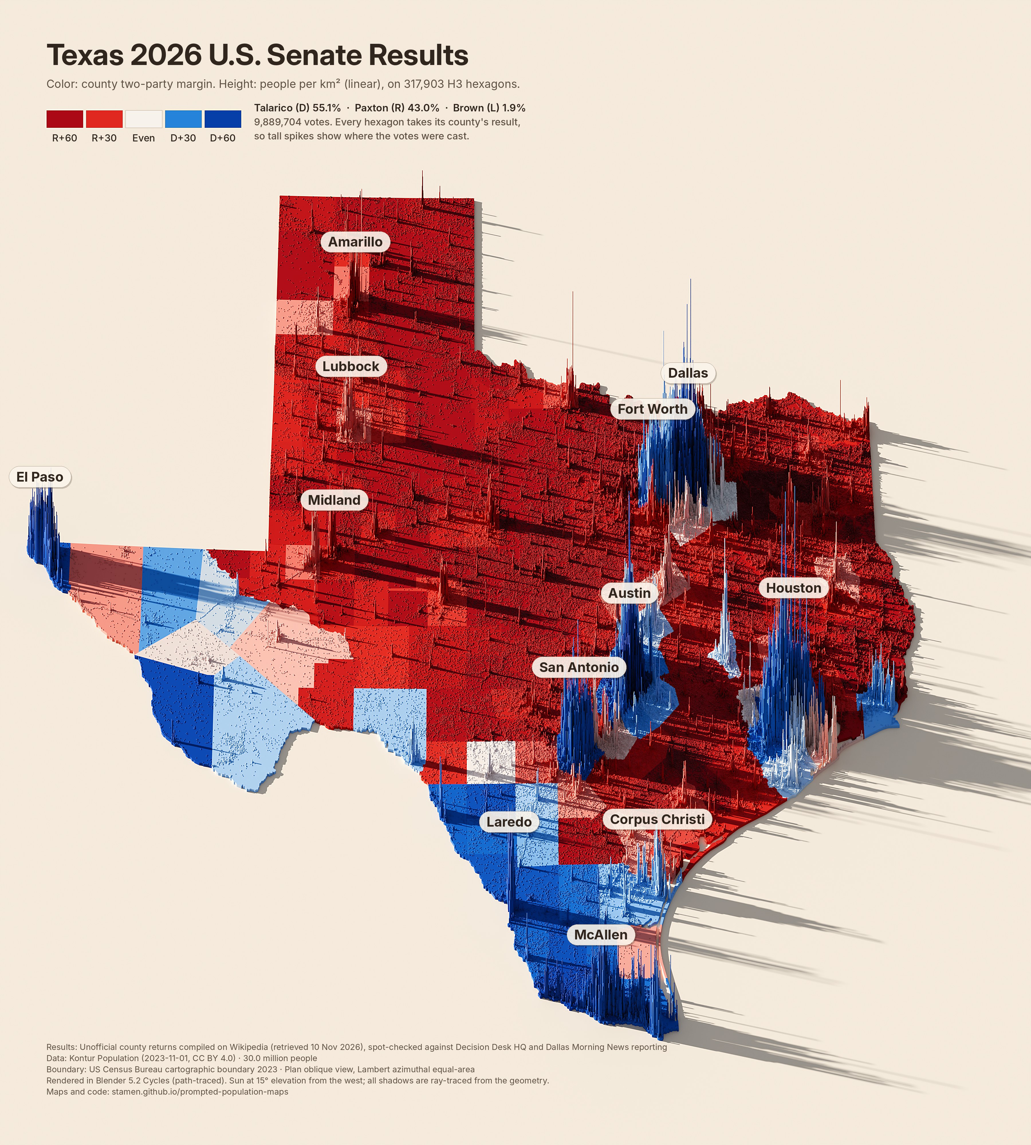
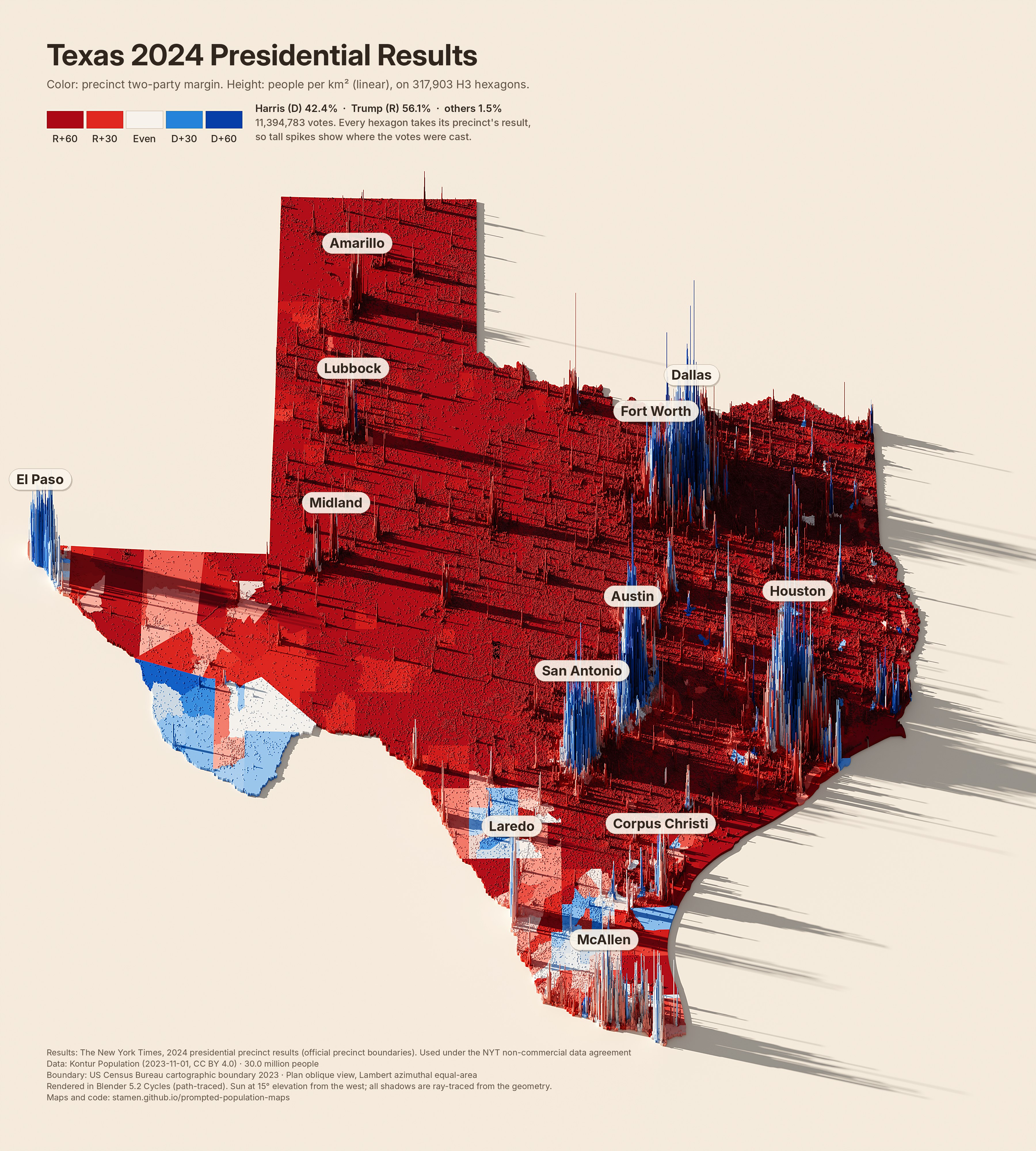
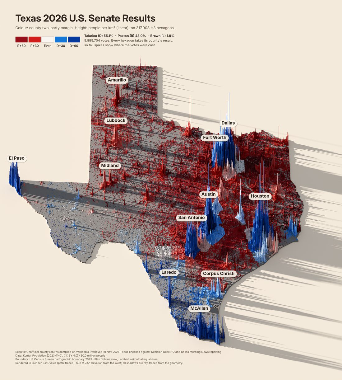
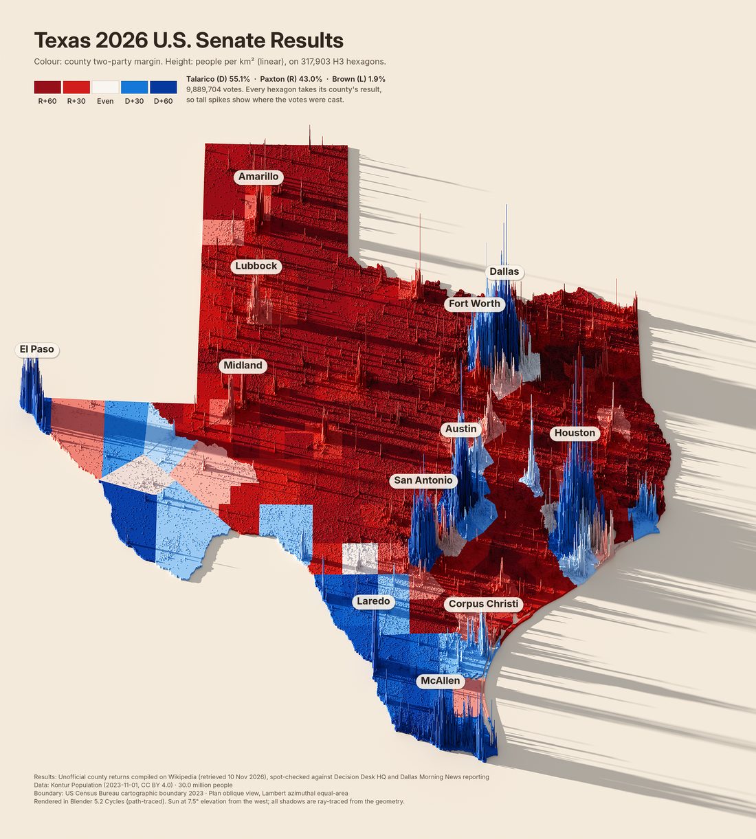
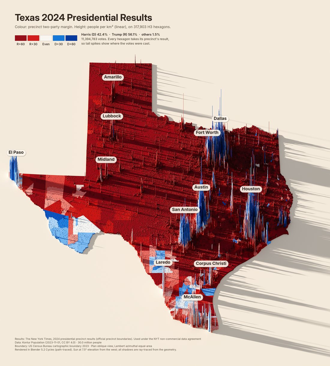
So, I was curious if we could color these with election results instead? Here is one using county-level results from the 2026 Senate election (precinct-level results are not available yet) and another with the 2024 presidential results to see what finer-grained precinct-level results will look like. The maps are certainly more complex and messy, but that’s what the real world is like:
— Alan
Votes on population
Election results draped on the same spikes
The height is still people per km². The color is the two-party margin of the county or precinct each hexagon falls in, from R+60 (dark red) to D+60 (dark blue), so the tall spikes show where the votes were cast.
2026 Senate: unofficial county returns compiled on Wikipedia (retrieved 10 Nov 2026), spot-checked against Decision Desk HQ and the Dallas Morning News; statewide precinct results were not yet published. 2024 presidential: The New York Times precinct results with official boundaries, used under the NYT non-commercial data agreement.
In the author's words
How these were made
I also wanted to be fully transparent about the process I used to make these maps. These were done via “prompting only,” per today’s #30DayMapChallenge rule. I told Claude what I wanted, gave it some specific direction about what data to include and what tools to use, and then spent several prompts iterating on the results.
In terms of creative control, there are certainly some decisions that Claude made that I didn’t bother to reconsider, but my goal was to use the AI for the tedious, uncreative work and keep most creative decisions for myself. As you can see in the prompts below, the initial result was really not ready for prime time. Claude needed a lot of human input to get the results into something more usable and visually pleasing.
— Alan
How we got here
Texas, prompt by prompt
The style was developed on Texas through a conversation with an AI coding agent. Each step shows the image, what was asked for, and what changed in the code.
First test render
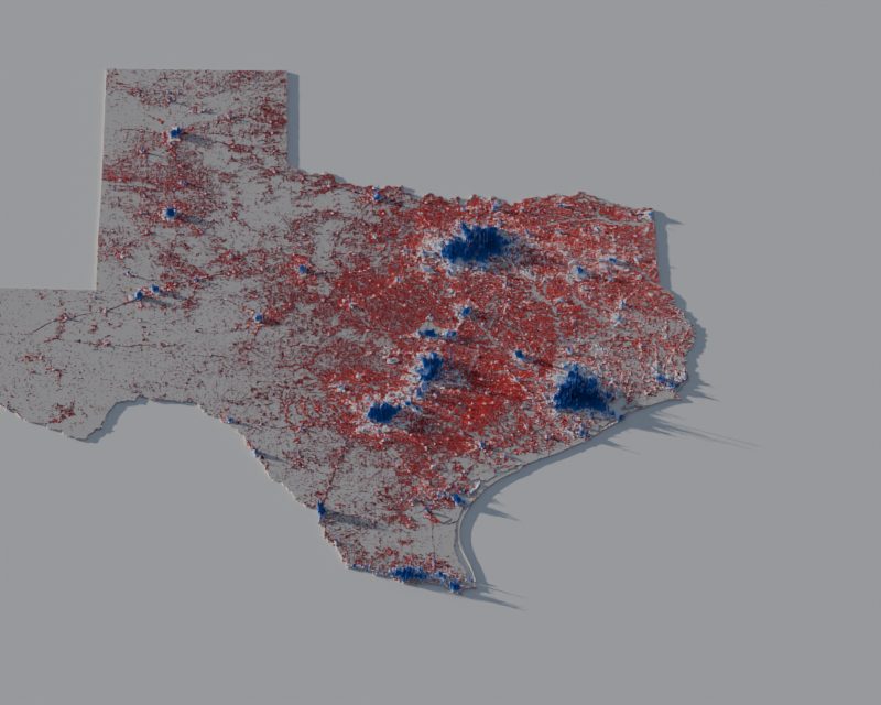
“Give me a population density map of Texas using gridded Kontur population data where each grid cell is extruded into the third dimension to show height. Add dramatic raytraced shadows… in the style of Blender, Aerialod, or R’s Rayshader plugin. Use a red-white-blue color scheme… Use real data, and real shadows, do not fake anything.”
An 800 px, 16-sample check of the pipeline: 317,903 Kontur hexagons became 2.2 million faces and path-traced in 8 seconds. Peaks were capped at 42 km and the base was light gray, so it read as flat and the white middle class blended into the base.
First full render
“(first delivered map)”
Peaks raised to 110 km and the sun lowered to 7.5° from the west-northwest so shadows run east across the state. Charcoal base, gray ground, gradient legend, title “Where 30 million people live”.
Brighter, taller, warmer, labeled
“Trim the scale so the zero point is a brighter red and the top is a brighter blue… boost the vertical scale… lighten and warm up the background… add annotation for the major city spikes.”
Darkest ends of the ramp trimmed, peaks to 180 km, sand ground, and twelve cities with leader lines and peak densities. Labels anchor on the visible skyline (25th-tallest nearby cell) because the densest cell is an invisible needle.
Uninhabited land in red
“The gray near-zero population background of the map should be red too.”
Kontur only lists inhabited hexagons, so empty land showed the base slab. The slab took the exact color of the lowest class.
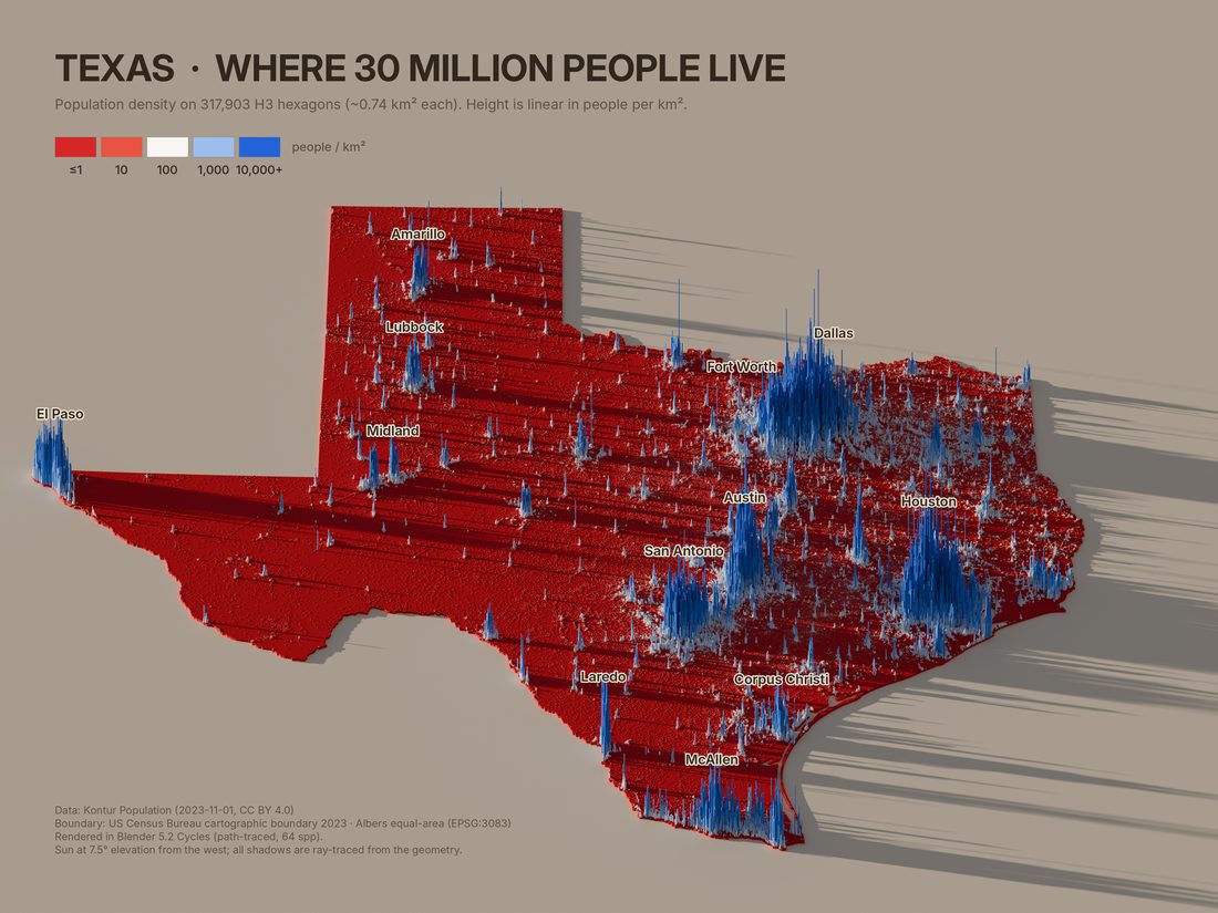
Names only, five swatches
“Remove the density numbers… remove the leader lines… boost the vertical scale even more… simplify the legend into just 5 swatches.”
Peaks to 280 km (2.5× the first render), plain names on each skyline, five swatches at 1, 10, 100, 1,000, and 10,000+ people per km².
Plan oblique view
“Stretch the image vertically so the image is closer to the proportions of Texas as viewed top down, but keep the perspective view.”
Blender renders with wide pixels (aspect 1/cos 50°): the ground keeps its top-down shape while heights still rise at the 50° view. Lighting is untouched and label positions come from Blender’s own camera projection.
Simpler title and a color grade
“Change the title to a simpler ‘Texas Population Density’… contrast, brightness, or other levels adjustments… bright and clean-looking.”
Levels put the sand near white, a gentle S-curve kept shadows strong, grays were neutralized, and reds pulled back from neon. Legend swatches are rendered as flat tiles under the map’s lighting so they match after the grade.
Readable labels and a stepped legend
“The place labels need adjustment so they’re a bit easier to read. Also the scale needs an extra callout… or make each swatch a different height.”
Bold names on cream pills with a faint outline and shadow. The swatches rise one step per 10×, with callouts: darkest blue is 10,000× denser than darkest red, and heights are linear (the tallest spike’s real value is printed).
2026 Senate results draped on population
“Source county level election results from the 2026 Texas US Senate race and drape those colors on the population map instead of coloring by density.”
254-county results (Wikipedia, spot-checked against Decision Desk HQ and the Dallas Morning News). Each hexagon takes its county’s two-party margin; uninhabited land is neutral gray.
County-colored land
“In this case I would color the slab according the county election results, too.”
The land slab is built from the 254 Census county polygons, each in its result color, so empty counties read correctly and spikes show where the votes are.
Precinct-level 2024 results
“Search the web for better resolution results, like at the precinct level… you can probably find it for the 2024 presidential results.”
2026 precinct data is not yet published statewide, so this uses the NYT’s 9,718 Texas precincts for 2024 (totals within 0.1% of certified). Cities split into blue cores and red suburbs; the Rio Grande Valley shows the 2024 shift.
Sun at 15°, centered labels
“Your city labels aren't correctly centered in their white background pill shapes… bring [the light] up higher above the horizon, try 15º.”
Names are centered on cap height. Shadows are half as long. The grade now measures the bare ground in each render, so the background stays the same cream at any sun angle.
Pick up where we left off
Make your own map
Clone the repo and either hand it to your own coding agent, or run the commands yourself. AGENTS.md tells any LLM (Claude, Codex, Gemini, Cursor, and others) how the pipeline works, what not to break, and how to check its work.
A prompt for your agent
Clone https://github.com/stamen/prompted-population-maps and read AGENTS.md.
Set up the environment, then make a population density map of Japan in the same style:
add a region entry, render a preview, show it to me, and check the population total
against the official figure before rendering the final.
Set up once
git clone https://github.com/stamen/prompted-population-maps
cd prompted-population-maps
uv venv -p 3.13 renv
uv pip install -p renv/bin/python -r requirements.txt
export PYTHON=renv/bin/python
pipeline/fetch_data.sh US DE        # ISO-2 codes you need
Blender installs from PyPI as bpy; no Blender app needed. Kontur files come from Kontur's public S3 bucket; boundaries from Natural Earth and the US Census.
Make a map
pipeline/make_map.sh germany preview   # ~30 s
pipeline/make_map.sh germany final     # 6–15 min
python docs/build_site.py              # refresh this site
Previews are 800 px at 16 samples; finals are 3600 px at 64 samples on 4 CPU cores. Iterate on previews, render the final once.
Where each style setting lives
To change
File
Look for
A region, its cities, its data
pipeline/regions.py
one entry in R
Sun height and direction
pipeline/regions.py
SUN_EL, SUN_AZ. Lower elevation means longer shadows
Density color ramp
pipeline/render.py, pipeline/legend_render.py
stops, cols. Change both, then re-run legend_render.py
Election color ramp
pipeline/regions.py
EL_STOPS, EL_COLS
Height exaggeration
pipeline/render.py
HMAX=0.224*S (S = region extent in km)
View tilt
pipeline/render.py, pipeline/legend_render.py
tilt; pixel_aspect_x = 1/cos(tilt) gives the plan-oblique view
Ground and uninhabited land color
pipeline/render.py
mat('ground', …), slabm
Brightness, contrast, saturation
pipeline/annotate.py
grade(); the white point is measured from the bare ground
Title, legend, callouts, labels
pipeline/annotate.py
text blocks; label pills and collision list taken
Margins and framing
pipeline/render.py
fx0, fx1, fy0, fy1. Extra room on the east is for shadows
Lessons
Things that will bite you
The densest cell is a needle
A city's densest hexagon is one pixel wide and towers over the visible skyline. Labels anchor on the 25th-tallest cell nearby instead, which is where the eye sees the city.
H3 cells are not always hexagons
Resolution-7 cells that straddle an icosahedron face edge carry up to 10 boundary vertices. prep.py keeps the six sharpest corners; pentagons are padded to six.
Lakes need two polygons
Clip the population with the full provincial boundary and build the land from the lake-cut shape. Clipping data with 1:10m lake shorelines dropped 780,000 Ontario lakeshore residents.
Legend colors must be rendered
Lighting and tone mapping change how each color looks. The swatches are flat tiles rendered under the identical sun and sky, then put through the same grade as the map.
Dense countries look different
Germany, the UK, and India are blue almost everywhere because rural density is in the hundreds per km². England's 99th-percentile cell is a quarter of its maximum, so its field is uniformly tall. That is the data.
Check totals, and check sources
prep.py prints the population it kept: Texas 29.95M, Germany 83.5M, India 1.43B, China 1.43B all match official figures. Election totals were checked against certified or independently reported numbers.
In the author's words
Why count tokens?
I was also curious how much effort each part of the process took, so I asked Claude to estimate the token usage for each step, and for what it took to generate the additional maps once we had the workflow set up. I’m no expert in interpreting the token usage, and these aren’t a good metric of the real-world economic and environmental impact of LLM usage. But I am curious how these compare relative to the still-significant electricity usage of running an hours-long Blender render if I’d done all the setup myself. I was also curious about using these numbers to compare with the costs of “faking” these maps without real data (more on that below). Why do people ask LLMs to make fake versions of these maps, and why do they seem content with them? Is it just that the fakes are easier and quicker (and cheaper) to make than asking the LLM to do the real work?
One of the other concerns with LLMs is that they often have to figure things out from first principles again and again, which wastes water and electricity. Using the scripts and documentation in this repo (provided above), I hope that other users can get up and running with this semi-automated pipeline themselves (with or without AI help) without having to repeat so many steps from scratch.
— Alan
Cost
What it took
Everything here was made in one long session with an AI coding agent. The measured totals come from the session's usage record; the per-phase split is an estimate made during the work.
Measured, whole session
Metric
Value
Output tokens (written by the model, including reasoning)
295,743
Input tokens, not cached
52,773
Cache writes
1,531,745
Cache reads (the conversation re-read on every step)
112,707,657
API cost at list price
$40.75
As of 2026-11-11 01:58 UTC (whole session). Cache reads dominate: every tool call re-reads the conversation so far.
Texas: plan oblique, title, grade, rendered legend
~20k
Texas subtotal
~72k
Generalize the pipeline to any region
~13k
Seven regions: config, previews, fixes
~11.5k
Ontario lakes
~4.5k
Portable scripts and first shared page
~19k
Readable labels and stepped legend
~5k
2026 Senate results by county
~22k
County-colored land
~6k
Precinct search and 2024 precinct map
~18k
Sun at 15°, centered labels
~9k
Repo, agent guide, and Pages site
~30k
Seven vibes maps (no data, same renderer)
~35k
Chatbot comparison section
~8k
Real data for the seven vibes countries
~15k
US Great Lakes cut out
~3k
Author’s notes and page edits
~15k
Each additional region, once generalized
~2k
In dollars
At list API prices, the whole session cost about $41. Usage readings taken along the way split it roughly like this:
$13.41 for everything up to the repository: the first Texas map and its revisions, the seven other density maps, and both election maps.
About $3 to turn that work into this repository, its agent guide, and this site.
About $2 for the seven vibes maps, measured between two readings.
About $22 for everything after that: the real versions of the seven vibes countries, the comparison section, the author’s notes, and page edits. The seven real countries were a few dollars of that (an estimate; they could not be separated from the other work).
Later steps cost more than early ones even when they did less, because each step re-reads the whole conversation, which by then was over half a million tokens. The same seven countries made in a fresh session from this repository would cost a small fraction as much, which is the point of writing everything down. The renders themselves ran for roughly four and a half hours of 4-core CPU time in total.
The first map took about a quarter of the new tokens. Once the pipeline was general, a new region cost about 2k new tokens (one config entry plus reviewing one preview) and 4–15 minutes of rendering, against about 5k per country for the vibes versions.
Source
The code
The same files as in the repository, shown here for reading.
AGENTS.mdinstructions for coding agents · on GitHub
# AGENTS.md: working on prompted-population-maps

Instructions for any coding agent (Claude, Codex, Gemini, Cursor, aider, …) or person continuing this project.
Read this file, then `README.md`. Everything you need to reproduce or extend the maps is in this repo.

## What this repo makes

3D population maps: every inhabited H3 hexagon from Kontur Population is extruded to a height that is
**linear in people per km²**, then path-traced in Blender Cycles (via the `bpy` Python module) under a low sun,
so shadows are real ray-traced shadows. Color is either population density (log scale) or an election
result (two-party margin, county or precinct), draped over the same population geometry.

## Setup

```bash
uv venv -p 3.13 renv            # or: python3.13 -m venv renv
uv pip install -p renv/bin/python -r requirements.txt
export PYTHON=renv/bin/python
pipeline/fetch_data.sh US IN FR GB CN HK MO DE CA   # Kontur files by ISO-2 code + boundaries (~2.5 GB)
pipeline/fetch_data.sh --elections                  # optional: Texas election data
```

No Blender app is needed; `bpy` is Blender as a Python module. Rendering is CPU-only by default.

## Commands

```bash
pipeline/make_map.sh germany preview   # 800 px, 16 samples, ~20-45 s  -> out/germany_preview.png
pipeline/make_map.sh germany final     # 3600 px, 64 samples, 6-15 min on 4 cores -> out/germany.png
python docs/build_site.py              # rebuild the GitHub Pages site from out/*.png and pipeline/*
```

`make_map.sh` runs, in order: `legend_render.py` (swatch colors under the current sun), `prep.py` (only if
`work/<region>.npz` is missing), `render.py`, `annotate.py`. Delete `work/<region>.npz` after changing anything
that `prep.py` reads (boundaries, clipping, resolution, election data).

## Repo map

| Path | Role |
|---|---|
| `pipeline/regions.py` | **All per-map configuration**, paths, sun angle (`SUN_EL`, `SUN_AZ`), election color ramp |
| `pipeline/prep.py` | Clip Kontur cells to the boundary, aggregate to H3 res 7 for regions wider than 2,000 km, project (Lambert azimuthal equal-area), join election results, write `work/<region>.npz` |
| `pipeline/render.py` | Build the Blender scene (hex prisms, land slab, ground, sun, sky, plan-oblique camera), export label anchors, path-trace |
| `pipeline/annotate.py` | Color grade, title, legend, callouts, credits, city labels with collision avoidance |
| `pipeline/legend_render.py` | Render flat swatch tiles under the map's exact lighting so legend colors match the map |
| `pipeline/fetch_data.sh`, `fetch_tx_senate_2026.py` | Data downloads |
| `docs/` | GitHub Pages site (`index.html` is generated by `docs/build_site.py` from `docs/template.html`) |
| `fonts/` | Inter (SIL OFL 1.1), used by `annotate.py` |

## Adding a region

1. Add an entry to `R` in `pipeline/regions.py`. Copy a similar one:
   - `kontur`: ISO-2 codes of the Kontur files (fetch them with `fetch_data.sh`).
   - `bnd`: `('ne0', [Natural Earth ADMIN names])` for countries, `('ne1', 'Province')` for provinces
     (prep.py filters `admin=='Canada'`; generalize that filter for other countries), `('census', 'ST')` for US states.
   - `national=True` only when the Kontur file covers exactly that territory (keeps coastal cells with a 3 km buffer).
   - optional `bbox` (drop overseas territories), `lakes=True` (cut Natural Earth lakes from the land slab).
   - optional `top` (headroom above the region, default 0.22 of its extent) when tall spikes sit on the northern edge (Egypt, Mexico).
   - optional `res` to force a coarser H3 resolution when a scene is too big to render (the contiguous US at res 7 needs more than 14 GB).
   - optional `parts` for places drawn at one scale but moved closer (see `usa_full`): each part has its own Natural Earth names, bounding boxes, cities, and a `place` rule relative to an earlier part. `prep.py` hands these regions to `prep_composite.py`. Kontur's US file already includes PR, VI, GU, MP, and AS, so do not add their own files.
   - `cities`: `(name, lon, lat)` in label priority order; colliding labels are nudged, then dropped.
2. `pipeline/make_map.sh <region> preview` and **look at the image**.
3. Check the population total `prep.py` prints against an official figure. Within ~2% is normal.
4. Render `final`, then `python docs/build_site.py` if it should appear on the site.

## Election maps

Add `election=dict(...)` to a region (see `texas_senate` and `texas_pres2024`):
- `level='county'`: a CSV with columns `county,d,r,l,o,tot` plus Census county polygons (`counties`, `statefp`).
- `level='precinct'`: a GeoJSON of precinct polygons with vote columns (`dcol`, `rcol`, `totcol`) and a sibling CSV.
Each hexagon takes the result of the unit containing its center; the land slab is built from the unit polygons,
each in its own result color. Color = (D−R)/(D+R) on `EL_STOPS`/`EL_COLS` in `regions.py`.

## Invariants: do not break these

- **Use real data only.** Never invent, interpolate, or "fill in" populations or votes. If a source is unreachable, stop and say so.
- **Heights stay linear** in people per km² (normalized to each map's densest cell). Color carries the log scale.
- **Keep the density ramp in sync.** `stops`/`cols` appear in `render.py` and `legend_render.py`; change both,
  then re-run `legend_render.py` (make_map.sh does this). The election ramp lives once, in `regions.py`.
- **Legend swatches must be rendered**, not picked: lighting and AgX tone mapping change how albedo looks.
- **Shadows are ray-traced.** Do not add 2D drop shadows or painted shading to the map.
- **Credit sources** on the image (Kontur CC BY 4.0; Natural Earth; US Census; NYT for precinct data, which is
  licensed for non-commercial use only and must credit The New York Times).

## Pitfalls already solved (read before "fixing" them)

- A city's densest cell is a one-pixel needle; labels anchor on the 25th-tallest cell within ~1.6% of the extent.
- H3 res-7 cells on icosahedron edges have up to 10 vertices; `prep.py` keeps the 6 sharpest corners.
- Clip population with the full boundary, but build the land slab from the lake-cut shape (Ontario lost 780k people otherwise).
- Germany, the UK, India, and eastern China are blue nearly everywhere because rural density is in the hundreds per km². That is data.
- `annotate.py` sets the white point from the bare ground in each render, so any sun angle grades the same.
- Plan oblique = render the 50° oblique view with `pixel_aspect_x = 1/cos(50°)`; do not stretch images afterwards.

## Verifying a change

Render a preview of `texas` and one other region, open both images, and compare against `docs/img/`.
For data changes, compare printed totals with official sources. There is no unit-test suite; images are the test.
# One entry per map. cities: (name, lon, lat) in label-priority order.
import os
ROOT=os.path.dirname(os.path.dirname(os.path.abspath(__file__)))
DATA=os.environ.get('POPMAPS_DATA',os.path.join(ROOT,'data'))    # downloads (fetch_data.sh)
WORK=os.environ.get('POPMAPS_WORK',os.path.join(ROOT,'work'))    # intermediates + raw renders
OUT=os.environ.get('POPMAPS_OUT',os.path.join(ROOT,'out'))       # finished maps
FONTS=os.path.join(ROOT,'fonts')
os.makedirs(WORK,exist_ok=True); os.makedirs(OUT,exist_ok=True)
NE0=f'{DATA}/bnd/ne_10m_admin_0_countries.geojson'; NE1=f'{DATA}/bnd/ne_10m_admin_1_states_provinces.geojson'
LAKES=f'{DATA}/bnd/ne_10m_lakes.geojson'
CENSUS=f'zip://{DATA}/bnd/cb_2023_us_state_5m.zip'
K=f'{DATA}/kontur/'
SITE_URL='stamen.github.io/prompted-population-maps'   # printed in every map's credits
SUN_EL=15.0; SUN_AZ=282.0     # sun elevation above the horizon and azimuth (degrees); lower = longer shadows
# election ramp on two-party margin (D-R)/(D+R): -0.6 = R+60 ... +0.6 = D+60
EL_STOPS=[-0.6,-0.3,-0.1,0.0,0.1,0.3,0.6]
EL_COLS=[[165,15,30],[214,48,44],[240,160,145],[246,240,232],[150,185,235],[45,110,210],[15,50,160]]
R={
 'texas':dict(title='Texas',kontur=['US'],bnd=('census','TX'),national=False,credit='US Census Bureau cartographic boundary 2023',
   cities=[('Houston',-95.37,29.76),('Dallas',-96.80,32.78),('Fort Worth',-97.33,32.75),('San Antonio',-98.49,29.42),('Austin',-97.74,30.27),('El Paso',-106.44,31.76),('McAllen',-98.23,26.20),('Laredo',-99.51,27.51),('Corpus Christi',-97.40,27.80),('Lubbock',-101.86,33.58),('Amarillo',-101.83,35.22),('Midland',-102.08,32.00)]),
 'texas_senate':dict(title='Texas 2026 U.S. Senate',election=dict(level='county',dem='Talarico (D)',rep='Paxton (R)',third='Brown (L)',csv=f'{DATA}/election/tx_senate_2026_county.csv',counties=f'zip://{DATA}/bnd/cb_2023_us_county_5m.zip',statefp='48',
     source='Unofficial county returns compiled on Wikipedia (retrieved 10 Nov 2026), spot-checked against Decision Desk HQ and Dallas Morning News reporting'),kontur=['US'],bnd=('census','TX'),national=False,credit='US Census Bureau cartographic boundary 2023',
   cities=[('Houston',-95.37,29.76),('Dallas',-96.80,32.78),('Fort Worth',-97.33,32.75),('San Antonio',-98.49,29.42),('Austin',-97.74,30.27),('El Paso',-106.44,31.76),('McAllen',-98.23,26.20),('Laredo',-99.51,27.51),('Corpus Christi',-97.40,27.80),('Lubbock',-101.86,33.58),('Amarillo',-101.83,35.22),('Midland',-102.08,32.00)]),
 'texas_pres2024':dict(title='Texas 2024 Presidential',election=dict(level='precinct',dem='Harris (D)',rep='Trump (R)',third=None,
     geo=f'{DATA}/election/nyt/TX.geojson',dcol='votes_dem',rcol='votes_rep',totcol='votes_total',
     source='The New York Times, 2024 presidential precinct results (official precinct boundaries). Used under the NYT non-commercial data agreement'),kontur=['US'],bnd=('census','TX'),national=False,credit='US Census Bureau cartographic boundary 2023',
   cities=[('Houston',-95.37,29.76),('Dallas',-96.80,32.78),('Fort Worth',-97.33,32.75),('San Antonio',-98.49,29.42),('Austin',-97.74,30.27),('El Paso',-106.44,31.76),('McAllen',-98.23,26.20),('Laredo',-99.51,27.51),('Corpus Christi',-97.40,27.80),('Lubbock',-101.86,33.58),('Amarillo',-101.83,35.22),('Midland',-102.08,32.00)]),
 'new_york':dict(title='New York State',kontur=['US'],bnd=('census','NY'),national=False,
   credit='US Census Bureau cartographic boundary 2023',
   cities=[('New York City',-74.00,40.71),('Buffalo',-78.88,42.89),('Rochester',-77.61,43.16),('Syracuse',-76.15,43.05),('Albany',-73.76,42.65),('Binghamton',-75.91,42.10),('Utica',-75.23,43.10),('Ithaca',-76.50,42.44),('Plattsburgh',-73.45,44.70)]),
 'india':dict(title='India',kontur=['IN'],bnd=('ne0',['India']),national=True,credit='Natural Earth 1:10m (de facto boundaries)',
   cities=[('Mumbai',72.88,19.08),('Delhi',77.21,28.61),('Kolkata',88.36,22.57),('Chennai',80.27,13.08),('Bengaluru',77.59,12.97),('Hyderabad',78.49,17.39),('Ahmedabad',72.57,23.02),('Pune',73.86,18.52),('Jaipur',75.79,26.91),('Lucknow',80.95,26.85),('Patna',85.14,25.59),('Guwahati',91.74,26.14),('Srinagar',74.80,34.08),('Kochi',76.27,9.93)]),
 'france':dict(title='France',kontur=['FR'],bnd=('ne0',['France']),national=True,bbox=(-6,41,10,52),credit='Natural Earth 1:10m (metropolitan France)',
   cities=[('Paris',2.35,48.86),('Lyon',4.84,45.76),('Marseille',5.37,43.30),('Toulouse',1.44,43.60),('Nice',7.26,43.70),('Lille',3.06,50.63),('Bordeaux',-0.58,44.84),('Nantes',-1.55,47.22),('Strasbourg',7.75,48.58),('Rennes',-1.68,48.11),('Montpellier',3.88,43.61),('Ajaccio',8.74,41.93)]),
 'uk':dict(title='United Kingdom',kontur=['GB'],bnd=('ne0',['United Kingdom']),national=True,credit='Natural Earth 1:10m',
   cities=[('London',-0.13,51.51),('Birmingham',-1.90,52.49),('Manchester',-2.24,53.48),('Glasgow',-4.25,55.86),('Edinburgh',-3.19,55.95),('Liverpool',-2.98,53.41),('Leeds',-1.55,53.80),('Newcastle',-1.61,54.97),('Bristol',-2.59,51.45),('Belfast',-5.93,54.60),('Cardiff',-3.18,51.48),('Sheffield',-1.47,53.38),('Aberdeen',-2.10,57.15),('Plymouth',-4.14,50.38)]),
 'china':dict(title='China',kontur=['CN','HK','MO'],bnd=('ne0',['China','Hong Kong S.A.R.','Macao S.A.R']),national=True,
   credit='Natural Earth 1:10m (de facto boundaries; includes Hong Kong & Macau)',
   cities=[('Shanghai',121.47,31.23),('Beijing',116.40,39.90),('Guangzhou',113.26,23.13),('Shenzhen',114.06,22.54),('Chongqing',106.55,29.56),('Chengdu',104.07,30.57),('Wuhan',114.31,30.59),("Xi'an",108.94,34.34),('Tianjin',117.20,39.13),('Harbin',126.53,45.80),('Hong Kong',114.17,22.32),('Kunming',102.83,24.88),('Shenyang',123.43,41.80),('Ürümqi',87.62,43.83),('Lhasa',91.13,29.65),('Lanzhou',103.83,36.06)]),
 'ontario':dict(title='Ontario',kontur=['CA'],bnd=('ne1','Ontario'),national=False,lakes=True,credit='Natural Earth 1:10m (lakes removed)',
   cities=[('Toronto',-79.38,43.65),('Ottawa',-75.70,45.42),('Hamilton',-79.87,43.26),('London',-81.25,42.98),('Windsor',-83.03,42.31),('Kitchener',-80.49,43.45),('Sudbury',-80.99,46.49),('Thunder Bay',-89.25,48.38),('Kingston',-76.48,44.23),('Sault Ste. Marie',-84.33,46.52),('Timmins',-81.33,48.48),('Moosonee',-80.65,51.27)]),
 'germany':dict(title='Germany',kontur=['DE'],bnd=('ne0',['Germany']),national=True,credit='Natural Earth 1:10m',
   cities=[('Berlin',13.40,52.52),('Hamburg',9.99,53.55),('Munich',11.58,48.14),('Cologne',6.96,50.94),('Frankfurt',8.68,50.11),('Stuttgart',9.18,48.78),('Düsseldorf',6.77,51.23),('Leipzig',12.37,51.34),('Dresden',13.74,51.05),('Hanover',9.73,52.37),('Nuremberg',11.08,49.45),('Bremen',8.80,53.08),('Dortmund',7.47,51.51)]),
 # ---- the seven countries first made "with vibes" (see the site), now from real data
 'usa':dict(title='United States (contiguous)',kontur=['US'],bnd=('ne0',['United States of America']),national=True,res=6,lakes=True,bbox=(-125,24,-66.5,49.5),credit='Natural Earth 1:10m (contiguous 48 states, lakes removed)',
   cities=[('New York',-74.0,40.7),('Los Angeles',-118.24,34.05),('Chicago',-87.63,41.88),('Houston',-95.37,29.76),('Dallas',-96.8,32.78),('Miami',-80.19,25.77),('Atlanta',-84.39,33.75),('Seattle',-122.33,47.61),('Denver',-104.99,39.74),('Phoenix',-112.07,33.45),('San Francisco',-122.42,37.77),('Minneapolis',-93.27,44.98)]),
 'russia':dict(title='Russia',kontur=['RU'],bnd=('ne0',['Russia']),national=True,bbox=(19,41,180,82),credit='Natural Earth 1:10m (de facto boundaries; Chukotka east of 180° omitted)',
   cities=[('Moscow',37.62,55.75),('St Petersburg',30.32,59.94),('Novosibirsk',82.92,55.03),('Yekaterinburg',60.6,56.84),('Kazan',49.11,55.79),('Rostov-on-Don',39.7,47.23),('Krasnoyarsk',92.87,56.01),('Omsk',73.37,54.99),('Irkutsk',104.3,52.29),('Vladivostok',131.89,43.12),('Khabarovsk',135.07,48.48),('Yakutsk',129.73,62.03)]),
 'japan':dict(title='Japan',kontur=['JP'],bnd=('ne0',['Japan']),national=True,bbox=(122,24,146.5,46),credit='Natural Earth 1:10m (remote Pacific islands omitted)',
   cities=[('Tokyo',139.69,35.69),('Osaka',135.5,34.69),('Nagoya',136.91,35.18),('Fukuoka',130.4,33.59),('Sapporo',141.35,43.06),('Sendai',140.87,38.27),('Hiroshima',132.46,34.39),('Niigata',139.04,37.92),('Kagoshima',130.56,31.6),('Naha',127.68,26.21),('Kanazawa',136.65,36.56),('Kochi',133.53,33.56)]),
 'mexico':dict(title='Mexico',kontur=['MX'],bnd=('ne0',['Mexico']),national=True,top=0.32,bbox=(-117.5,14,-86,33),credit='Natural Earth 1:10m (remote Pacific islands omitted)',
   cities=[('Mexico City',-99.13,19.43),('Guadalajara',-103.35,20.67),('Monterrey',-100.31,25.69),('Puebla',-98.2,19.04),('Tijuana',-117.04,32.51),('León',-101.68,21.12),('Juárez',-106.42,31.69),('Mérida',-89.62,20.97),('Chihuahua',-106.09,28.63),('Culiacán',-107.39,24.8),('Acapulco',-99.82,16.86),('Cancún',-86.85,21.16)]),
 'brazil':dict(title='Brazil',kontur=['BR'],bnd=('ne0',['Brazil']),national=True,bbox=(-74.5,-34,-34,5.5),credit='Natural Earth 1:10m (Atlantic islands omitted)',
   cities=[('São Paulo',-46.63,-23.55),('Rio de Janeiro',-43.2,-22.9),('Belo Horizonte',-43.94,-19.92),('Brasília',-47.88,-15.79),('Salvador',-38.5,-12.97),('Fortaleza',-38.54,-3.72),('Recife',-34.88,-8.05),('Porto Alegre',-51.23,-30.03),('Curitiba',-49.27,-25.43),('Manaus',-60.02,-3.12),('Belém',-48.5,-1.46),('Goiânia',-49.25,-16.68)]),
 'australia':dict(title='Australia',kontur=['AU'],bnd=('ne0',['Australia']),national=True,bbox=(112,-44,154,-9),credit='Natural Earth 1:10m (external territories omitted)',
   cities=[('Sydney',151.21,-33.87),('Melbourne',144.96,-37.81),('Brisbane',153.03,-27.47),('Perth',115.86,-31.95),('Adelaide',138.6,-34.93),('Canberra',149.13,-35.28),('Hobart',147.33,-42.88),('Darwin',130.84,-12.46),('Townsville',146.82,-19.26),('Cairns',145.77,-16.92),('Alice Springs',133.88,-23.7),('Newcastle',151.78,-32.93)]),
 'egypt':dict(title='Egypt',kontur=['EG'],bnd=('ne0',['Egypt']),national=True,top=0.55,credit='Natural Earth 1:10m (de facto boundaries)',
   cities=[('Cairo',31.24,30.04),('Alexandria',29.92,31.2),('Port Said',32.3,31.26),('Suez',32.55,29.97),('Mansoura',31.38,31.04),('Tanta',31.0,30.79),('Asyut',31.18,27.18),('Luxor',32.64,25.69),('Aswan',32.9,24.09),('Hurghada',33.81,27.26),('Siwa',25.52,29.2),('Marsa Matruh',27.24,31.35)]),
 # ---- the whole United States at one scale: each part keeps its own true size and shape, moved closer (prep_composite.py).
 #      Kontur's US file already includes PR, VI, GU, MP, and AS; adding their own files would double-count them.
 'usa_full':dict(title='United States',kontur=['US'],national=True,res=6,lakes=True,bnd=None,
   credit='Natural Earth 1:10m (lakes removed). Alaska, Hawaii, and the territories are moved closer but drawn at the same scale',
   cities=[],
   parts=[
    dict(name='Contiguous US',ne=['United States of America'],bbox=[(-125,24,-66.5,49.5)],
         cities=[('New York',-74.0,40.7),('Los Angeles',-118.24,34.05),('Chicago',-87.63,41.88),('Houston',-95.37,29.76),('Dallas',-96.8,32.78),('Miami',-80.19,25.77),('Atlanta',-84.39,33.75),('Seattle',-122.33,47.61),('Denver',-104.99,39.74),('Phoenix',-112.07,33.45),('San Francisco',-122.42,37.77),('Minneapolis',-93.27,44.98)]),
    dict(name='Alaska',ne=['United States of America'],bbox=[(-180,51,-129,72),(172,51,180,54)],west_of_180=True,
         place=dict(ref='Contiguous US',x='left_of',y='align_top',dy=500),cities=[('Anchorage',-149.9,61.22),('Fairbanks',-147.72,64.84),('Juneau',-134.42,58.3)]),
    dict(name='Hawaii',ne=['United States of America'],bbox=[(-161,18.5,-154.5,22.5)],
         place=dict(ref='Alaska',x='align_right',y='below'),cities=[('Honolulu',-157.86,21.31)]),
    dict(name='Guam and Northern Mariana Islands',ne=['Guam','Northern Mariana Islands'],bbox=[(144,13,146.5,21)],
         place=dict(ref='Hawaii',x='left_of',y='align_top'),cities=[('Hagåtña',144.75,13.47)]),
    dict(name='American Samoa',ne=['American Samoa'],bbox=[(-171.2,-14.6,-168,-11)],
         place=dict(ref='Hawaii',x='align_right',y='below'),cities=[('Pago Pago',-170.70,-14.28)]),
    dict(name='Puerto Rico and US Virgin Islands',ne=['Puerto Rico','United States Virgin Islands'],bbox=[(-68,17.5,-64.5,18.6)],
         place=dict(ref='Contiguous US',x='align_right',y='below',dx=-700),cities=[('San Juan',-66.1,18.47)]),
   ]),
}
pipeline/prep.pyclip, aggregate, project, join elections · on GitHub
import os, sys, numpy as np, pandas as pd, pyogrio, h3, geopandas as gpd, shapely, time
from shapely.ops import unary_union
from pyproj import Transformer
import os; sys.path.insert(0,os.path.dirname(os.path.abspath(__file__))); from regions import *
key=sys.argv[1]; c=R[key]; t=time.time()
if 'parts' in c:   # several places at one scale (e.g. the full US): see prep_composite.py
    import runpy; runpy.run_path(os.path.join(os.path.dirname(os.path.abspath(__file__)),'prep_composite.py'),run_name='__main__'); sys.exit()
b=c['bnd']
if b[0]=='census': g=gpd.read_file(CENSUS); g=g[g.STUSPS==b[1]].to_crs(4326).geometry
elif b[0]=='ne0': g=gpd.read_file(NE0); g=g[g.ADMIN.isin(b[1])].geometry
else: g=gpd.read_file(NE1); g=g[(g['name']==b[1])&(g.admin=='Canada')].geometry
geom=unary_union(list(g))
if 'bbox' in c: geom=geom.intersection(shapely.box(*c['bbox']))
if c.get('lakes'):   # cut out the Great Lakes and inland lakes so the land mass follows the real shoreline
    lk=gpd.read_file(LAKES); lk=lk[lk.intersects(geom)].geometry; land=geom.difference(unary_union(list(lk))).buffer(0)
else: land=geom
df=pd.concat([pyogrio.read_dataframe(K+f+'.gpkg',read_geometry=False,columns=['h3','population']) for f in c['kontur']])
lon0,lat0=(geom.bounds[0]+geom.bounds[2])/2,(geom.bounds[1]+geom.bounds[3])/2
tr=Transformer.from_crs(4326,f'+proj=laea +lat_0={lat0} +lon_0={lon0} +units=km',always_xy=True)
gp=shapely.ops.transform(lambda x,y:tr.transform(x,y),geom)
gl=shapely.ops.transform(lambda x,y:tr.transform(x,y),land)
S=max(gp.bounds[2]-gp.bounds[0],gp.bounds[3]-gp.bounds[1])
res=c.get('res') or (8 if S<=2000 else 7)   # 'res' overrides (e.g. 6 for the contiguous US, which needs >14 GB to render at res 7)
cells=df.h3.values; pop=df.population.values.astype(float)
if res<8:   # sum Kontur res-8 populations into their res-7 parents (real totals, coarser cells)
    par=np.array([h3.cell_to_parent(x,res) for x in cells]); s=pd.Series(pop).groupby(par).sum(); cells=s.index.values; pop=s.values
ll=np.array([h3.cell_to_latlng(x) for x in cells])
clip=gp.buffer(3.0) if c['national'] else gp    # national files contain only that country: small buffer keeps coastal cells
X,Y=tr.transform(ll[:,1],ll[:,0]); keep=shapely.contains_xy(clip,X,Y)
cells,pop=cells[keep],pop[keep]
def bnd6(x):
    v=h3.cell_to_boundary(x)
    if len(v)>6:   # icosahedron-edge cells carry extra near-collinear 'distortion' vertices: keep the 6 sharpest corners
        a=np.array(v); d1=a-np.roll(a,1,0); d2=np.roll(a,-1,0)-a
        ang=np.abs(np.arctan2(d1[:,0]*d2[:,1]-d1[:,1]*d2[:,0],(d1*d2).sum(1)))
        v=tuple(map(tuple,a[np.sort(np.argsort(-ang)[:6])]))
    return v if len(v)==6 else v+(v[-1],)*(6-len(v))
verts=np.array([bnd6(x) for x in cells]); vx,vy=tr.transform(verts[...,1],verts[...,0])
area=np.array([h3.cell_area(x,'km^2') for x in cells])
cx,cy=(gp.bounds[0]+gp.bounds[2])/2,(gp.bounds[1]+gp.bounds[3])/2
parts=[p for p in (gl.geoms if gl.geom_type=='MultiPolygon' else [gl]) if p.area>max(20,S*S*2e-5)]
polys=np.empty(len(parts),object); polys[:]=[np.array(p.simplify(S/4000).exterior.coords)-[cx,cy] for p in parts]
extra={}
if 'election' in c:
    E=c['election']
    if E['level']=='county':   # county table joined to Census county polygons by name
        er=pd.read_csv(E['csv']); er['m']=(er.d-er.r)/(er.d+er.r)
        co=gpd.read_file(E['counties']); co=co[co.STATEFP==E['statefp']].merge(er,left_on='NAME',right_on='county').to_crs(4326)
    else:                      # precinct polygons that already carry vote counts
        co=gpd.read_file(E['geo']).to_crs(4326); co['m']=(co[E['dcol']]-co[E['rcol']])/(co[E['dcol']]+co[E['rcol']]).clip(lower=1)
        co['geometry']=co.geometry.buffer(0)
    lat_,lon_=np.array([h3.cell_to_latlng(x) for x in cells]).T
    pts=gpd.GeoDataFrame(geometry=gpd.points_from_xy(lon_,lat_),crs=4326)
    j=gpd.sjoin_nearest(pts.to_crs(3083),co[['m','geometry']].to_crs(3083),how='left').groupby(level=0).first()   # nearest handles edge cells
    # county-colored slab: triangulate each county (holes/islands kept) and keep its outline rings for walls
    ct,ctm,cr,crm=[],[],[],[]
    for g_,m_ in zip(co.geometry,co.m):
        gq=shapely.ops.transform(lambda x,y:tr.transform(x,y),g_)
        for p_ in (gq.geoms if gq.geom_type=='MultiPolygon' else [gq]):
            q=p_.simplify(S/4000 if E['level']=='county' else S/25000)   # precincts are tiny in cities: simplify gently
            if q.is_empty or q.area<0.0005: continue
            if not q.is_valid: q=q.buffer(0)
            if q.geom_type!='Polygon': continue
            for t_ in shapely.constrained_delaunay_triangles(q).geoms: ct.append(np.array(t_.exterior.coords)[:3]-[cx,cy]); ctm.append(m_)
            for r_ in [q.exterior,*q.interiors]: cr.append(np.array(r_.coords)-[cx,cy]); crm.append(m_)
    extra['ctris']=np.array(ct); extra['ctm']=np.array(ctm); rr=np.empty(len(cr),object); rr[:]=cr; extra['crings']=rr; extra['crm']=np.array(crm)
    print('county slab triangles',len(ct))
    extra['margin']=j['m'].values; print('cells per county ok; margin range',np.nanmin(extra['margin']).round(3),np.nanmax(extra['margin']).round(3))
if c.get('lakes'):   # triangulate the slab with holes (inland lakes), plus every ring for the side walls
    tris=[];rings=[]
    for p in parts:
        q=p.simplify(S/4000)
        for t_ in shapely.constrained_delaunay_triangles(q).geoms: tris.append(np.array(t_.exterior.coords)[:3]-[cx,cy])
        rings+= [np.array(q.exterior.coords)-[cx,cy]]+[np.array(r.coords)-[cx,cy] for r in q.interiors]
    rr=np.empty(len(rings),object); rr[:]=rings; extra=dict(tris=np.array(tris),rings=rr)
    print('slab triangles',len(tris),'rings',len(rings))
np.savez(f'{WORK}/{key}.npz',**extra,x=vx-cx,y=vy-cy,pop=pop,area=area,polys=polys,proj=np.array([lon0,lat0,cx,cy]),
         bounds=np.array(gp.bounds)-[cx,cy,cx,cy],res=res)
print(f'{key}: res{res} cells={len(cells)} pop={pop.sum():,.0f} extent={S:.0f}km polys={len(parts)} maxdens={np.max(pop/area):,.0f} {time.time()-t:.0f}s')
pipeline/render.pybuild scene and path-trace · on GitHub
# usage: render.py <region> <width_px> <spp> <out.png>   (height is derived from the region's plan-oblique frame)
import bpy, bmesh, numpy as np, math, sys, time, json
from mathutils import Vector
from bpy_extras.object_utils import world_to_camera_view
import os; sys.path.insert(0,os.path.dirname(os.path.abspath(__file__))); from regions import R, WORK
key,WPX,SPP,OUT=sys.argv[1],int(sys.argv[2]),int(sys.argv[3]),sys.argv[4]
d=np.load(f'{WORK}/{key}.npz',allow_pickle=True); c=R[key]
X,Y=d['x'],d['y']; dens=d['pop']/d['area']; n=len(dens)
x0,y0,x1,y1=d['bounds']; S=max(x1-x0,y1-y0)          # all dimensions scale from the Texas design (S=1250 km)
HMAX=0.224*S; h=0.0002*S+dens/dens.max()*HMAX; SLAB=0.0024*S
# color: same absolute log-density ramp as Texas, so maps are comparable
ld=np.log10(np.clip(dens,1,None)); stops=np.array([0.0,1.0,1.8,2.6,3.4,4.15])
cols=np.array([[215,38,40],[232,84,66],[250,246,240],[244,246,250],[70,135,225],[25,90,215]])/255.
rgb=np.stack([np.interp(ld,stops,cols[:,k]) for k in range(3)],1)
if 'margin' in d.files:   # color = county two-party margin (D-R)/(D+R): red Republican, blue Democratic
    from regions import EL_STOPS, EL_COLS
    ec=np.array(EL_COLS)/255.; rgb=np.stack([np.interp(d['margin'],EL_STOPS,ec[:,k]) for k in range(3)],1)
lin=np.where(rgb<=0.04045,rgb/12.92,((rgb+0.055)/1.055)**2.4)
V=np.stack([np.concatenate([X,X],1),np.concatenate([Y,Y],1),np.concatenate([np.repeat(h[:,None],6,1),np.zeros((n,6))],1)],-1).reshape(-1,3)
base=(np.arange(n)*12)[:,None]; top=base+np.arange(6)[None,:]
sides=np.stack([np.stack([base[:,0]+a,base[:,0]+6+a,base[:,0]+6+(a+1)%6,base[:,0]+(a+1)%6],1) for a in range(6)],1)
loops=np.concatenate([top,sides.reshape(n,24)],1).reshape(-1); sizes=np.tile([6,4,4,4,4,4,4],n); starts=np.concatenate([[0],np.cumsum(sizes)[:-1]])
bpy.ops.wm.read_factory_settings(use_empty=True); s=bpy.context.scene
me=bpy.data.meshes.new('hex'); me.vertices.add(len(V)); me.vertices.foreach_set('co',V.astype(np.float32).ravel())
me.loops.add(len(loops)); me.loops.foreach_set('vertex_index',loops.astype(np.int32))
me.polygons.add(len(sizes)); me.polygons.foreach_set('loop_start',starts.astype(np.int32)); me.polygons.foreach_set('loop_total',sizes.astype(np.int32))
me.update(calc_edges=True); me.validate()
at=me.attributes.new('col','FLOAT_COLOR','FACE'); at.data.foreach_set('color',np.repeat(np.concatenate([lin,np.ones((n,1))],1),7,0).astype(np.float32).ravel())
ob=bpy.data.objects.new('hex',me); s.collection.objects.link(ob); bpy.context.view_layer.objects.active=ob; ob.select_set(True)
bpy.ops.object.mode_set(mode='EDIT'); bpy.ops.mesh.select_all(action='SELECT'); bpy.ops.mesh.normals_make_consistent(inside=False); bpy.ops.object.mode_set(mode='OBJECT')
def mat(name,color=None,attr=None,rough=0.55):
    m=bpy.data.materials.new(name); m.use_nodes=True; p=m.node_tree.nodes['Principled BSDF']; p.inputs['Roughness'].default_value=rough
    if attr: a=m.node_tree.nodes.new('ShaderNodeAttribute'); a.attribute_name=attr; m.node_tree.links.new(a.outputs['Color'],p.inputs['Base Color'])
    else: p.inputs['Base Color'].default_value=(*color,1)
    return m
ob.data.materials.append(mat('hexm',attr='col'))
slabm=mat('slab',(0.30,0.27,0.24) if 'margin' in d.files else (0.680,0.019,0.021),rough=0.8)      # uninhabited: neutral for election maps, lowest red class for density
def elcol(m):   # election ramp in linear RGB
    from regions import EL_STOPS, EL_COLS
    ec=np.array(EL_COLS)/255.; r=np.stack([np.interp(m,EL_STOPS,ec[:,k]) for k in range(3)],-1)
    return np.where(r<=0.04045,r/12.92,((r+0.055)/1.055)**2.4)
if 'ctris' in d.files:   # election maps: slab built from county polygons, each in its county's result color
    T=d['ctris']; nt=len(T); C=elcol(d['ctm'])
    vt=[np.dstack([T,np.zeros((nt,3,1))]).reshape(-1,3),np.dstack([T,np.full((nt,3,1),-SLAB)]).reshape(-1,3)]
    ft=[(3*i,3*i+1,3*i+2) for i in range(nt)]+[(3*(nt+i)+2,3*(nt+i)+1,3*(nt+i)) for i in range(nt)]; fc=list(C)+list(C)
    o_=2*3*nt
    for Rg,m_ in zip(d['crings'],elcol(d['crm'])):
        k_=len(Rg)-1; vt.append(np.vstack([np.c_[Rg[:-1],np.zeros(k_)],np.c_[Rg[:-1],np.full(k_,-SLAB)]]))
        ft+=[(o_+i,o_+(i+1)%k_,o_+k_+(i+1)%k_,o_+k_+i) for i in range(k_)]; fc+=[m_]*k_; o_+=2*k_
    sm=bpy.data.meshes.new('cslab'); sm.from_pydata(np.vstack(vt).tolist(),[],ft); sm.update()
    a_=sm.attributes.new('col','FLOAT_COLOR','FACE'); a_.data.foreach_set('color',np.c_[np.array(fc),np.ones(len(fc))].astype(np.float32).ravel())
    so_=bpy.data.objects.new('cslab',sm); s.collection.objects.link(so_); sm.materials.append(mat('cslabm',attr='col',rough=0.8))
    bpy.context.view_layer.objects.active=so_; bpy.ops.object.mode_set(mode='EDIT'); bpy.ops.mesh.select_all(action='SELECT')
    bpy.ops.mesh.normals_make_consistent(inside=False); bpy.ops.object.mode_set(mode='OBJECT')
elif 'tris' in d.files:   # hole-aware slab (lakes cut out): triangulated top/bottom + walls on every ring
    T=d['tris']; nt=len(T); vt=np.concatenate([np.dstack([T,np.zeros((nt,3,1))]),np.dstack([T,np.full((nt,3,1),-SLAB)])]).reshape(-1,3)
    ft=[(3*i,3*i+1,3*i+2) for i in range(nt)]+[(3*(nt+i)+2,3*(nt+i)+1,3*(nt+i)) for i in range(nt)]
    for Rg in d['rings']:
        o_=len(vt); m_=len(Rg)-1; ring=np.vstack([np.c_[Rg[:-1],np.zeros(m_)],np.c_[Rg[:-1],np.full(m_,-SLAB)]]); vt=np.vstack([vt,ring])
        ft+=[(o_+i,o_+(i+1)%m_,o_+m_+(i+1)%m_,o_+m_+i) for i in range(m_)]
    sm=bpy.data.meshes.new('slab'); sm.from_pydata(vt.tolist(),[],ft); sm.update(); sm.validate()
    so_=bpy.data.objects.new('slab',sm); s.collection.objects.link(so_); sm.materials.append(slabm)
    bpy.context.view_layer.objects.active=so_; bpy.ops.object.mode_set(mode='EDIT'); bpy.ops.mesh.select_all(action='SELECT')
    bpy.ops.mesh.remove_doubles(threshold=1e-4); bpy.ops.mesh.normals_make_consistent(inside=False); bpy.ops.object.mode_set(mode='OBJECT')
for k,P in enumerate([] if ('tris' in d.files or 'ctris' in d.files) else d['polys']):
    sm=bpy.data.meshes.new(f's{k}'); bm=bmesh.new(); vs=[bm.verts.new((px,py,0.0)) for px,py in P[:-1]]
    try: f=bm.faces.new(vs)
    except Exception: bm.free(); continue
    r=bmesh.ops.extrude_face_region(bm,geom=[f]); bmesh.ops.translate(bm,verts=[e for e in r['geom'] if isinstance(e,bmesh.types.BMVert)],vec=(0,0,-SLAB))
    bmesh.ops.recalc_face_normals(bm,faces=bm.faces); bm.to_mesh(sm); bm.free()
    so_=bpy.data.objects.new(f's{k}',sm); s.collection.objects.link(so_); sm.materials.append(slabm)
bpy.ops.mesh.primitive_plane_add(size=6*S,location=(0,0,-SLAB)); bpy.context.object.data.materials.append(mat('ground',(0.92,0.72,0.50),rough=0.9))
sun=bpy.data.lights.new('sun','SUN'); sun.energy=6.0; sun.angle=math.radians(0.6); sun.color=(1.0,0.93,0.84)
so=bpy.data.objects.new('sun',sun); s.collection.objects.link(so); from regions import SUN_EL, SUN_AZ; el,az=math.radians(SUN_EL),math.radians(SUN_AZ)
so.rotation_euler=Vector((math.sin(az)*math.cos(el),math.cos(az)*math.cos(el),math.sin(el))).to_track_quat('Z','Y').to_euler()
w=bpy.data.worlds.new('w'); s.world=w; w.use_nodes=True
w.node_tree.nodes['Background'].inputs['Color'].default_value=(0.55,0.65,0.85,1); w.node_tree.nodes['Background'].inputs['Strength'].default_value=0.35
# ---- plan-oblique frame: margins for shadows (east), title (top) and credits (bottom)
fx0,fx1,fy0,fy1=x0-0.03*S,x1+0.13*S,y0-0.12*S,y1+c.get('top',0.22)*S   # 'top': extra headroom when tall spikes sit on the northern edge
FW,FH=fx1-fx0,fy1-fy0; HPX=int(round(WPX*FH/FW))
if HPX>int(WPX*1.4): WPX=int(round(WPX*1.4*FW/FH)); HPX=int(round(WPX*FH/FW))   # cap very tall frames
tilt=math.radians(50); D=4*S
cam=bpy.data.cameras.new('cam'); cam.type='ORTHO'; cam.ortho_scale=FW; cam.sensor_fit='HORIZONTAL'; cam.clip_end=20*S
co=bpy.data.objects.new('cam',cam); s.collection.objects.link(co); s.camera=co
co.location=((fx0+fx1)/2,(fy0+fy1)/2-D*math.sin(tilt),D*math.cos(tilt)); co.rotation_euler=(tilt,0,0)
s.render.resolution_x=WPX; s.render.resolution_y=HPX; s.render.resolution_percentage=100
s.render.pixel_aspect_x=1/math.cos(tilt); s.render.pixel_aspect_y=1.0; bpy.context.view_layer.update()
# ---- label anchors: each city's visible skyline (25th-tallest cell within ~1.6% of extent)
from pyproj import Transformer
lon0,lat0,pcx,pcy=d['proj']; tr=Transformer.from_crs(4326,f'+proj=laea +lat_0={lat0} +lon_0={lon0} +units=km',always_xy=True)
CX,CY=X.mean(1),Y.mean(1); lab=[]; rad=max(12,0.016*S)
cities_xy=[tuple(q) for q in d['city_xy']] if 'city_xy' in d.files else [(n_,*(np.array(tr.transform(lo,la))-[pcx,pcy])) for n_,lo,la in c['cities']]
for name,ex,ey in cities_xy:
    m=np.where((CX-ex)**2+(CY-ey)**2<rad**2)[0]
    if len(m)==0: print('no cells near',name); continue
    sky=np.sort(h[m])[-min(25,len(m))]; j=m[np.argmin(np.abs(h[m]-sky))]
    # label sits at the city's own coordinates, raised to its visible skyline height
    v=world_to_camera_view(s,co,Vector((ex,ey,h[j]))); lab.append((name,v.x*WPX,(1-v.y)*HPX))
parts_lab=[]
for name,px_,py_ in (d['part_xy'] if 'part_xy' in d.files else []):   # caption under each moved part of a composite map
    v=world_to_camera_view(s,co,Vector((px_,py_,0))); parts_lab.append((name,v.x*WPX,(1-v.y)*HPX))
meta=dict(parts=parts_lab,labels=lab,cells=int(n),res=int(d['res']),cell_km2=float(np.median(d['area'])),pop=float(d['pop'].sum()))
json.dump(meta,open(OUT.rsplit('.',1)[0]+'_meta.json','w'))
if os.environ.get('POPMAPS_LABELS_ONLY'): sys.exit(0)   # recompute label anchors without rendering
s.render.engine='CYCLES'; s.cycles.device='CPU'; s.cycles.samples=SPP; s.cycles.use_denoising=True; s.cycles.max_bounces=4
s.view_settings.view_transform='AgX'; s.view_settings.look='AgX - Medium High Contrast'
s.render.image_settings.file_format='PNG'; s.render.filepath=OUT
t=time.time(); bpy.ops.render.render(write_still=True); print(f'{key} {WPX}x{HPX} render {time.time()-t:.0f}s faces {len(me.polygons)}')
pipeline/annotate.pygrade, title, legend, labels · on GitHub
# usage: annotate.py <region> <raw.png> <out.png>
import numpy as np, sys, json, os
from PIL import Image, ImageDraw, ImageFont, ImageFilter
sys.path.insert(0,os.path.dirname(os.path.abspath(__file__))); from regions import R, WORK, SUN_EL, FONTS, SITE_URL
from pyproj import Transformer
key,RAW,OUT=sys.argv[1:4]; c=R[key]; meta=json.load(open(RAW.rsplit('.',1)[0]+'_meta.json'))
def ground_level(im):
    a=np.asarray(im).astype(np.float32); W_,H_=im.size; g=a[int(H_*0.01):int(H_*0.06),int(W_*0.85):int(W_*0.99)].max(2).ravel()
    return float(np.median(g[g>=np.median(g)]))
def grade(im,wp):
    a=np.asarray(im).astype(np.float32)/255
    a=np.clip(a/(wp/255),0,1); a=np.clip(a-0.10*np.sin(2*np.pi*a)/np.pi,0,1)**1.03
    l=a@np.array([0.2126,0.7152,0.0722],np.float32); sat=a.max(2)-a.min(2)
    f=np.where(sat<0.22,0.55,1.0-0.10*np.clip((sat-0.22)/0.4,0,1))
    a=np.clip(l[...,None]+(a-l[...,None])*f[...,None],0,1)*np.array([1.0,0.99,0.965],np.float32)
    im=Image.fromarray((np.clip(a,0,1)*255+0.5).astype(np.uint8))
    return im.filter(ImageFilter.UnsharpMask(radius=max(1,im.size[0]/1800),percent=55,threshold=2))
raw=Image.open(RAW).convert('RGB'); WP=ground_level(raw)*1.024; W,H=raw.size; U=0.75*min(W,H*0.857)
F=FONTS+'/'
fT=ImageFont.truetype(F+'InterDisplay-Bold.otf',int(U*0.040)); fS=ImageFont.truetype(F+'Inter-Regular.otf',int(U*0.0155))
fL=ImageFont.truetype(F+'Inter-Medium.otf',int(U*0.0135)); fLb=ImageFont.truetype(F+'Inter-SemiBold.otf',int(U*0.0140))
fC=ImageFont.truetype(F+'Inter-Regular.otf',int(U*0.0115)); fN=ImageFont.truetype(F+'Inter-Bold.otf',int(U*0.0185))
ink=(48,38,30); sub=(95,82,68); cream=(250,244,234)
mx,my=int(W*0.045),int(U*0.05)
if 'election' in c:
    # ---- election legend: 5 equal swatches on the two-party margin, plus the statewide result
    E=c['election']; import pandas as pd
    if E['level']=='county': er=pd.read_csv(E['csv']); T=dict(d=er.d.sum(),r=er.r.sum(),l=er.l.sum(),tot=er.tot.sum())
    else: er=pd.read_csv(E['geo'].replace('.geojson','.csv')); T=dict(d=er[E['dcol']].sum(),r=er[E['rcol']].sum(),l=0,tot=er[E['totcol']].sum())
    T=pd.Series(T)
    sw,gap,sh=int(U*0.05),int(U*0.004),int(U*0.024); yb=my+int(U*0.10)+sh
    d0=ImageDraw.Draw(raw)
    for n,col in enumerate(json.load(open(f'{WORK}/legend_colors_election.json'))):
        x=mx+n*(sw+gap); d0.rectangle([x,yb-sh,x+sw,yb],fill=tuple(int(q) for q in col))
    im=grade(raw,WP); dr=ImageDraw.Draw(im)
    dr.text((mx,my),f"{c['title']} Results",font=fT,fill=ink)
    dr.text((mx,my+int(U*0.055)),f"Color: {E['level']} two-party margin. Height: people per km² (linear), on 317,903 H3 hexagons.",font=fS,fill=sub)
    for n,lab in enumerate(['R+60','R+30','Even','D+30','D+60']):
        x=mx+n*(sw+gap); dr.rectangle([x,yb-sh,x+sw,yb],outline=(175,160,140),width=1)
        w=dr.textlength(lab,font=fL); dr.text((x+sw/2-w/2,yb+int(U*0.006)),lab,font=fL,fill=ink)
    lx2=mx+5*(sw+gap)+int(U*0.014); y=yb-sh-int(U*0.012)
    pc=lambda v:f"{v/T.tot*100:.1f}%"
    head=f"{E['dem']} {pc(T.d)}  ·  {E['rep']} {pc(T.r)}"+(f"  ·  {E['third']} {pc(T.l)}" if E.get('third') else f"  ·  others {pc(T.tot-T.d-T.r)}")
    for t,f,col in [(head,fLb,ink),
                    (f"{T.tot:,.0f} votes. Every hexagon takes its {E['level']}'s result,",fL,sub),
                    ("so tall spikes show where the votes were cast.",fL,sub)]:
        dr.text((lx2,y),t,font=f,fill=col); y+=int(f.size*1.45)
    legend_bottom=max(y,yb+int(U*0.03))
else:
    # ---- legend: a staircase of the 5 classes (one step per 10x), bottom-aligned on a baseline
    sw,gap=int(U*0.05),int(U*0.004); step=int(U*0.011); base_h=int(U*0.014)
    yb=my+int(U*0.10)+base_h+4*step                                       # baseline of the stairs
    d0=ImageDraw.Draw(raw)
    for n,col in enumerate(json.load(open(f'{WORK}/legend_colors.json'))):  # swatch colors rendered under the map lighting
        x=mx+n*(sw+gap); d0.rectangle([x,yb-(base_h+n*step),x+sw,yb],fill=tuple(int(q) for q in col))
    im=grade(raw,WP); dr=ImageDraw.Draw(im)
    dr.text((mx,my),f"{c['title']} Population Density",font=fT,fill=ink)
    agg='' if meta['res']==8 else ', summed from Kontur res-8'
    dr.text((mx,my+int(U*0.055)),f"{meta['cells']:,} H3 hexagons (~{meta['cell_km2']:.2f} km² each{agg}). Height is linear in people per km².",font=fS,fill=sub)
    for n,lab in enumerate(['≤1','10','100','1,000','10,000+']):
        x=mx+n*(sw+gap); dr.rectangle([x,yb-(base_h+n*step),x+sw,yb],outline=(175,160,140),width=1)
        w=dr.textlength(lab,font=fL); dr.text((x+sw/2-w/2,yb+int(U*0.006)),lab,font=fL,fill=ink)
    lx2=mx+5*(sw+gap)+int(U*0.014); top=yb-(base_h+4*step)
    # callout: what the stairs mean, and what the spike heights mean
    d=np.load(f'{WORK}/{key}.npz',allow_pickle=True); dens=d['pop']/d['area']; i=int(np.argmax(dens))
    lon0,lat0,pcx,pcy=d['proj']; tr=Transformer.from_crs(4326,f'+proj=laea +lat_0={lat0} +lon_0={lon0} +units=km',always_xy=True)
    mxk,myk=d['x'][i].mean(),d['y'][i].mean()
    cxy=[tuple(q) for q in d['city_xy']] if 'city_xy' in d.files else [(n_,*(np.array(tr.transform(lo,la))-[pcx,pcy])) for n_,lo,la in c['cities']]
    near=min(cxy,key=lambda q:np.hypot(q[1]-mxk,q[2]-myk))[0]
    lines=[('Each color step is 10× denser',fLb,ink),
           ('Darkest blue (10,000+ people/km²) is 10,000× denser than darkest red (≤1).',fL,sub),
           (f'Spike height is linear: the tallest, in {near}, is {dens[i]:,.0f} people/km².',fL,sub)]
    y=top-int(U*0.002)
    for t,f,col in lines: dr.text((lx2,y),t,font=f,fill=col); y+=int(f.size*1.45)
    legend_bottom=max(y,yb+int(U*0.03))
cr=(f"Results: {c['election']['source']}\n" if 'election' in c else "")+f"Data: Kontur Population (2023-11-01, CC BY 4.0) · {meta['pop']/1e6:,.1f} million people\nBoundary: {c['credit']} · Plan oblique view, {meta.get('projection','Lambert azimuthal equal-area')}\nRendered in Blender 5.2 Cycles (path-traced). Sun at {SUN_EL:g}° elevation from the west; all shadows are ray-traced from the geometry."
cr+=f"\nMaps and code: {SITE_URL}"
dr.multiline_text((mx,H-my-int(U*(0.091 if 'election' in c else 0.073))),cr,font=fC,fill=sub,spacing=int(U*0.004))
# ---- city labels: bold name on a soft cream pill sitting just above each city's skyline
taken=[(0,0,W,legend_bottom+int(U*0.01)),(0,H-my-int(U*0.11),W,H)]
def hit(b): return any(not(b[2]<t[0] or b[0]>t[2] or b[3]<t[1] or b[1]>t[3]) for t in taken)
ov=Image.new('RGBA',im.size,(0,0,0,0)); do=ImageDraw.Draw(ov); texts=[]
capH=fN.getbbox('H')[3]-fN.getbbox('H')[1]; padx,pady=fN.size*0.55,fN.size*0.42
for name,px,py in meta['labels']:
    l_,t_,r_,b_=fN.getbbox(name,anchor='ls'); w=r_-l_; bw,bh=w+2*padx,capH+2*pady
    # Nudges never move a label off its spike: straight up (one or two steps) first, then sideways by less than half the pill's
    # width (so the pill still covers its anchor), then both. If nothing fits, the label is dropped, not misplaced.
    for dx,dy in [(0,0),(0,-1.1),(0,-2.2),(0.3,0),(-0.3,0),(0.3,-1.1),(-0.3,-1.1)]:
        x=px-bw/2+dx*bw; y=py-U*0.010-bh+dy*bh; b=(x-3,y-3,x+bw+3,y+bh+3)
        if not hit(b): break
    else:
        print(f'  label dropped (no room): {name}'); continue
    if (dx,dy)!=(0,0): print(f'  label nudged {"up" if dy else ""}{" " if dx and dy else ""}{"right" if dx>0 else "left" if dx<0 else ""}: {name}')
    taken.append(b)
    do.rounded_rectangle([x+U*0.0012,y+U*0.0018,x+bw+U*0.0012,y+bh+U*0.0018],radius=bh/2,fill=(40,28,18,55))   # soft drop shadow
    do.rounded_rectangle([x,y,x+bw,y+bh],radius=bh/2,fill=(*cream,232),outline=(150,128,104,200),width=max(1,int(U/1400)))
    texts.append((x+bw/2-(l_+r_)/2,y+bh/2+capH/2,name))         # baseline so capitals sit centered; ink box centered horizontally
for name,px,py in meta.get('parts',[]):   # composite maps: small caption under each moved part
    w=dr.textlength(name,font=fL); dr.text((px-w/2,py+U*0.008),name,font=fL,fill=sub)
ov=ov.filter(ImageFilter.GaussianBlur(0)) ; im=Image.alpha_composite(im.convert('RGBA'),ov).convert('RGB'); dr=ImageDraw.Draw(im)
for x,y,name in texts: dr.text((x,y),name,font=fN,fill=ink,anchor='ls')
im.save(OUT,optimize=True)
pipeline/legend_render.pyrender the swatch colors · on GitHub
# Render the 5 legend swatches as flat tiles under the identical material, sun, sky, and AgX settings as render.py,
# so each swatch shows exactly how a flat hexagon top of that density class appears in the map.
import bpy, numpy as np, math, sys, json
from mathutils import Vector
import os; sys.path.insert(0,os.path.dirname(os.path.abspath(__file__))); from regions import WORK
MODE=sys.argv[1] if len(sys.argv)>1 else 'density'
OUT=f'{WORK}/legend_colors.json' if MODE=='density' else f'{WORK}/legend_colors_election.json'
stops=np.array([0.0,1.0,1.8,2.6,3.4,4.15]); cols=np.array([[215,38,40],[232,84,66],[250,246,240],[244,246,250],[70,135,225],[25,90,215]])/255.
bpy.ops.wm.read_factory_settings(use_empty=True); s=bpy.context.scene
for n,v in enumerate([0,1,2,3,4]):
    if MODE=='election':
        from regions import EL_STOPS, EL_COLS
        rgb=np.array([np.interp([-0.6,-0.3,0,0.3,0.6][n],EL_STOPS,np.array(EL_COLS)[:,k]/255.) for k in range(3)])
    else: rgb=np.array([np.interp(v,stops,cols[:,k]) for k in range(3)])
    rgb=rgb; lin=np.where(rgb<=0.04045,rgb/12.92,((rgb+0.055)/1.055)**2.4)
    bpy.ops.mesh.primitive_plane_add(size=1.0,location=(n*1.5,0,0)); ob=bpy.context.object
    m=bpy.data.materials.new(f'm{n}'); m.use_nodes=True; p=m.node_tree.nodes['Principled BSDF']
    p.inputs['Roughness'].default_value=0.55; p.inputs['Base Color'].default_value=(*lin,1); ob.data.materials.append(m)
sun=bpy.data.lights.new('sun','SUN'); sun.energy=6.0; sun.angle=math.radians(0.6); sun.color=(1.0,0.93,0.84)
so=bpy.data.objects.new('sun',sun); s.collection.objects.link(so)
from regions import SUN_EL, SUN_AZ; elev=math.radians(SUN_EL); az=math.radians(SUN_AZ)
so.rotation_euler=Vector((math.sin(az)*math.cos(elev),math.cos(az)*math.cos(elev),math.sin(elev))).to_track_quat('Z','Y').to_euler()
w=bpy.data.worlds.new('w'); s.world=w; w.use_nodes=True
w.node_tree.nodes['Background'].inputs['Color'].default_value=(0.55,0.65,0.85,1); w.node_tree.nodes['Background'].inputs['Strength'].default_value=0.35
cam=bpy.data.cameras.new('c'); cam.type='ORTHO'; cam.ortho_scale=7.5; co=bpy.data.objects.new('c',cam); s.collection.objects.link(co); s.camera=co
tilt=math.radians(50); co.location=(3.0,-10*math.sin(tilt),10*math.cos(tilt)); co.rotation_euler=(tilt,0,0)   # same view angle as the map
s.render.engine='CYCLES'; s.cycles.samples=64; s.cycles.use_denoising=True; s.cycles.max_bounces=4
s.render.resolution_x=750; s.render.resolution_y=150
s.view_settings.view_transform='AgX'; s.view_settings.look='AgX - Medium High Contrast'
s.render.filepath=f'{WORK}/legend_tiles.png'; bpy.ops.render.render(write_still=True)
from PIL import Image
a=np.asarray(Image.open(f'{WORK}/legend_tiles.png').convert('RGB')).astype(float)
res=[a[70:80,int((n*1.5-3.0+3.75)/7.5*750)-5:int((n*1.5-3.0+3.75)/7.5*750)+5].reshape(-1,3).mean(0).round().tolist() for n in range(5)]
json.dump(res,open(OUT,'w')); print(res)
pipeline/make_map.shone command per map · on GitHub
#!/usr/bin/env bash
# One command per map.   pipeline/make_map.sh <region> [preview|final]
#   preview: 800 px, 16 samples (~20 s)     final: 3600 px, 64 samples (6-15 min on 4 CPU cores)
set -euo pipefail
HERE="$(cd "$(dirname "$0")" && pwd)"; PY="${PYTHON:-python}"; K="$1"; MODE="${2:-preview}"
WORK="${POPMAPS_WORK:-$HERE/../work}"; OUT="${POPMAPS_OUT:-$HERE/../out}"; mkdir -p "$WORK" "$OUT"
if [ "$MODE" = final ]; then W=3600; S=64; DST="$OUT/$K.png"; else W=800; S=16; DST="$OUT/${K}_preview.png"; fi
"$PY" "$HERE/legend_render.py" >/dev/null; "$PY" "$HERE/legend_render.py" election >/dev/null   # swatches under the current sun
[ -s "$WORK/$K.npz" ] || "$PY" "$HERE/prep.py" "$K"
"$PY" "$HERE/render.py" "$K" $W $S "$WORK/${K}_${MODE}_raw.png" 2>&1 | grep -E "render [0-9]|Error|Traceback" || true
"$PY" "$HERE/annotate.py" "$K" "$WORK/${K}_${MODE}_raw.png" "$DST"
echo "wrote $DST"
#!/usr/bin/env bash
# Download inputs into ./data (override with POPMAPS_DATA).
#   pipeline/fetch_data.sh US IN FR GB CN HK MO DE CA     Kontur population files by ISO-2 code
#   pipeline/fetch_data.sh --elections                    Texas 2026 Senate (county) + 2024 presidential (precinct)
set -euo pipefail
HERE="$(cd "$(dirname "$0")" && pwd)"; D="${POPMAPS_DATA:-$HERE/../data}"; mkdir -p "$D/kontur" "$D/bnd" "$D/election/nyt"
get(){ [ -s "$2" ] || { echo "-> $2"; curl -fSL --retry 3 -o "$2" "$1"; }; }
NE=https://raw.githubusercontent.com/nvkelso/natural-earth-vector/master/geojson
for f in ne_10m_admin_0_countries ne_10m_admin_1_states_provinces ne_10m_lakes; do get "$NE/$f.geojson" "$D/bnd/$f.geojson"; done
get https://www2.census.gov/geo/tiger/GENZ2023/shp/cb_2023_us_state_5m.zip  "$D/bnd/cb_2023_us_state_5m.zip"
get https://www2.census.gov/geo/tiger/GENZ2023/shp/cb_2023_us_county_5m.zip "$D/bnd/cb_2023_us_county_5m.zip"
for c in "$@"; do
  if [ "$c" = "--elections" ]; then
    python "$HERE/fetch_tx_senate_2026.py" "$D/election/tx_senate_2026_county.csv"
    for x in geojson csv; do get "https://int.nyt.com/newsgraphics/elections/map-data/2024/national/TX-precincts-with-results.$x.gz" "$D/election/nyt/TX.$x.gz"
      [ -s "$D/election/nyt/TX.$x" ] || gunzip -kf "$D/election/nyt/TX.$x.gz"; done
    continue
  fi
  # Kontur Population 2023-11-01, one GeoPackage per country (same files as on data.humdata.org)
  [ -s "$D/kontur/$c.gpkg" ] || { echo "-> kontur $c"; curl -fSL --retry 3 "https://geodata-eu-central-1-kontur-public.s3.amazonaws.com/kontur_datasets/kontur_population_${c}_20231101.gpkg.gz" | gunzip > "$D/kontur/$c.gpkg"; }
done
pipeline/fetch_tx_senate_2026.py2026 Senate county results · on GitHub
"""Texas 2026 U.S. Senate results by county, parsed from the Wikipedia article's county table.
Unofficial returns compiled from county reports; replace with the Secretary of State canvass when it is certified.
usage: python fetch_tx_senate_2026.py out.csv"""
import sys, io, urllib.request, pandas as pd
URL='https://en.wikipedia.org/w/index.php?title=2026_United_States_Senate_election_in_Texas&action=render'
html=urllib.request.urlopen(urllib.request.Request(URL,headers={'User-Agent':'prompted-population-maps'})).read().decode()
t=[t for t in pd.read_html(io.StringIO(html)) if len(t)>250 and t.astype(str).apply(lambda c:c.str.contains('Talarico')).any().any()][0]
t=t.iloc[:,:12]; t.columns=['county','d','dp','r','rp','l','lp','o','op','m','mp','tot']
num=lambda c: pd.to_numeric(t[c].astype(str).str.replace(',',''),errors='coerce')
for c in ['d','r','l','o','tot']: t[c]=num(c)
t=t[t.d.notna() & ~t.county.astype(str).str.contains('Total|County')]
assert len(t)==254, f'expected 254 counties, got {len(t)}'
assert (t.d+t.r+t.l+t.o==t.tot).all(), 'county columns do not add up'
t[['county','d','r','l','o','tot']].astype({'d':int,'r':int,'l':int,'o':int,'tot':int}).to_csv(sys.argv[1],index=False)
print(f"254 counties  D {t.d.sum():,.0f}  R {t.r.sum():,.0f}  total {t.tot.sum():,.0f} -> {sys.argv[1]}")
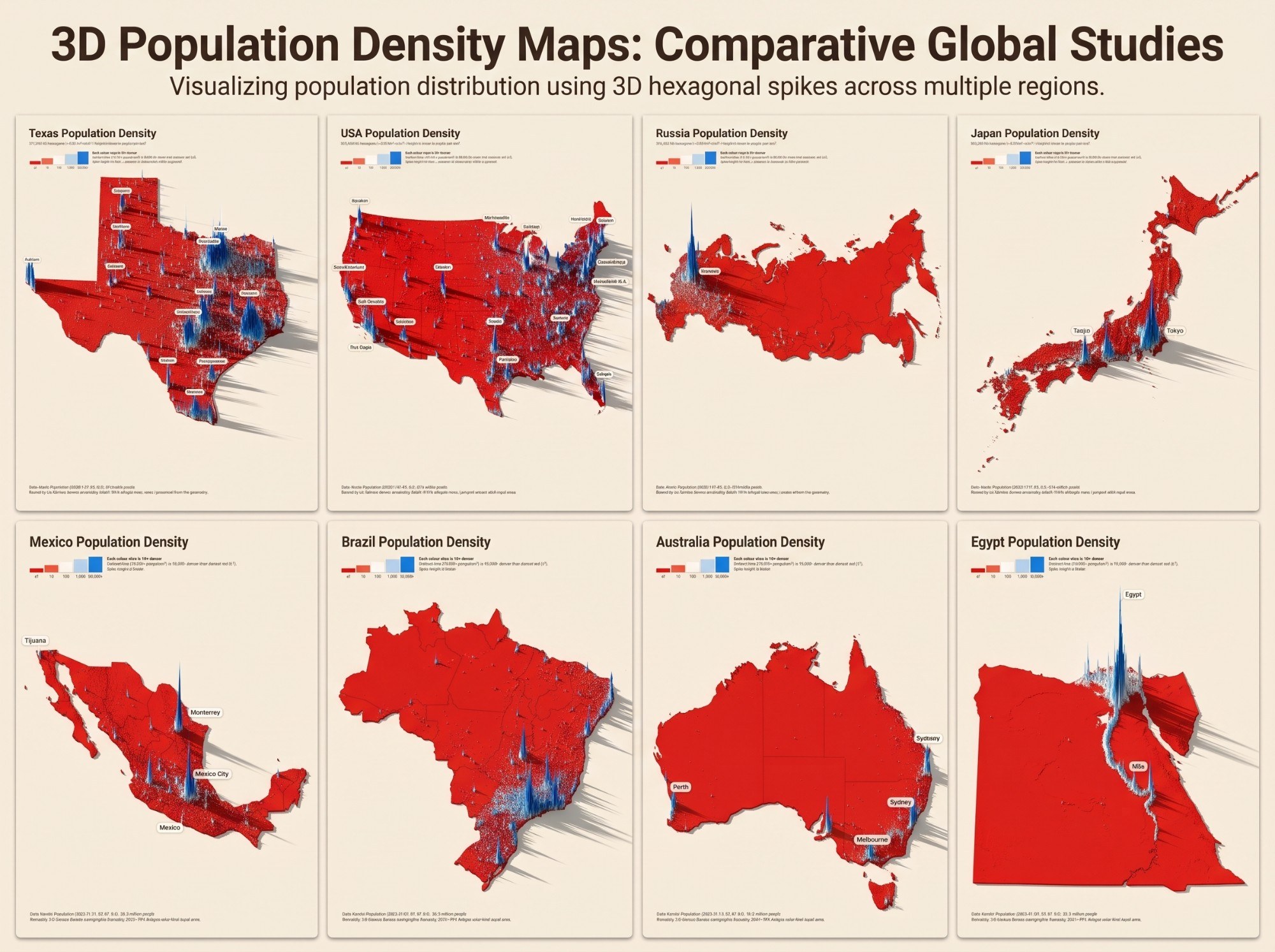
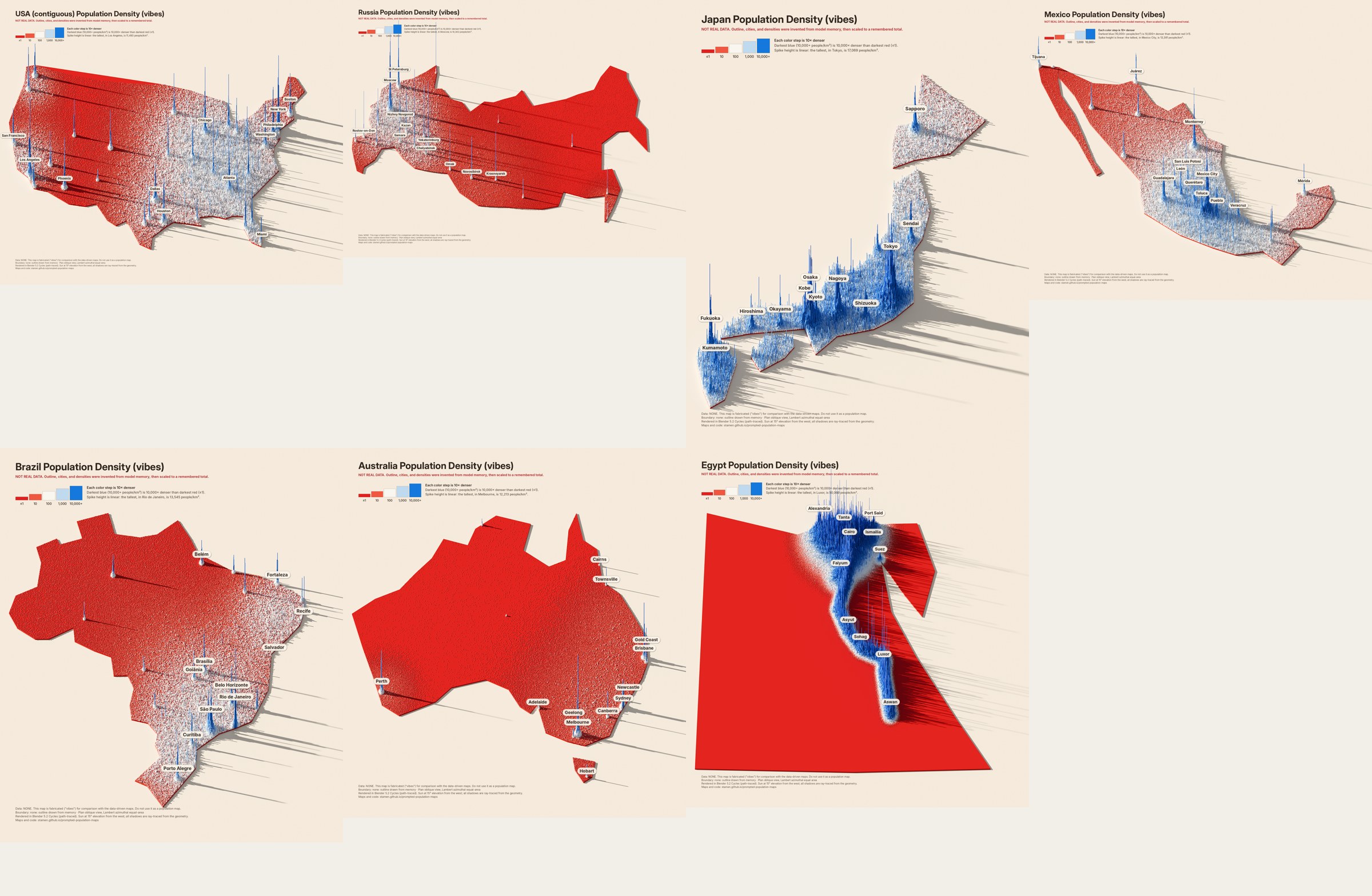
We gave ChatGPT and Gemini the final Texas map and one sentence, with no other context. Neither was asked to fake anything, and neither had population data. Both returned images that imitate the style: the spikes, colors, legend, and shadows are painted, not computed. The third example is this project's own agent, asked to fake the maps on purpose with code.
The exact prompt, with the Texas image attached
Here's a population density map of Texas. Make some in a similar style for the following countries: USA, Russia, Japan, Mexico, Brazil, Australia, Egypt
Response 1: Geminione image, eight panels, Texas redrawn alongside the seven countries
Almost every label is unreadable or invented: the Texas panel's city names are made-up words, Japan gets “Taqjio” beside Tokyo, and Egypt's tallest spike is labeled “Egypt.”
The small text (subtitles, legend callouts, credits) is letter-shaped noise that only resembles the Texas originals.
Russia is almost entirely flat red with one spike, and Brazil and Australia show internal borders that were never in the source style.
The overall look (cream ground, red land, blue spikes, long eastward shadows) is copied convincingly.
The labels are readable and mostly in the right places, which makes this the more convincing of the two chatbot images at a glance.
Each map carries a precise population and area, but nothing on the map was computed from them. The callout still says the tallest spike “is 13,394 people/km²,” which is Houston's value, copied from the Texas image.
The per-map legends repeat a swatch (“1,000” twice, and one reads “1:00”), and Egypt is drawn as a rectangle.
Density is painted where it feels right rather than where people live: Russia's far east, around Vladivostok, is as blue as Moscow.
Response 3 was asked for differently, in the same session that built this pipeline
Given this final style that we have settled on, can you make similar maps for some other countries (like, the USA, Russia, Japan, Mexico, Brazil, Australia, Egypt) but without using data. Just do it with vibes.
Response 3: Claude Code, faking it with codeinvented inputs, real renderer, labeled “NOT REAL DATA”
The inputs are invented, but the rendering is real. Outlines were typed from memory as rough coordinate lists, cities placed from memory with guessed metro sizes, rural density guessed as smooth regional patterns plus noise, and each map scaled to a remembered national total. The pipeline's own renderer then extruded and ray-traced it.
Because the text is set in code, every title, legend, and label is correct and readable, and every image says it is fabricated. That is the danger of this route: it looks exactly as authoritative as the real maps.
The tells are in the geography and the texture. Egypt is a trapezoid with the Sinai misplaced, Baja California is a wedge, and Japan's islands are blobs. The countryside is a smooth gradient instead of roads, rivers, and towns, and cities are symmetric needles.
Errors in the guesses do not announce themselves: Japan came out blue almost everywhere because the guessed rural density was too high.
Measured cost: about 30k output tokens (about $2.30) for all seven, plus about a minute of rendering each. That was cheap only because the real pipeline already existed; once it does, a real map costs about 2k tokens, less than a fake one.
Together they show why faking stays tempting: the look is the easy part to imitate, and the errors only show up when you check the geography, the numbers, and the text against a real source.
Back to real data
The same seven countries, for real
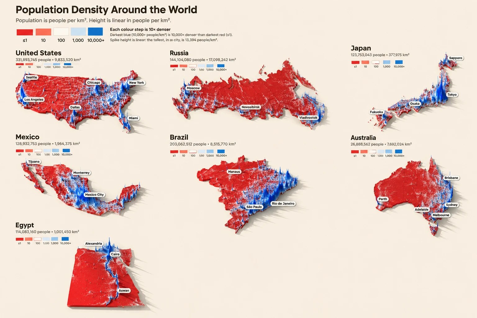
The same pipeline, run on the same seven countries with real data: Kontur population, Natural Earth boundaries, and nothing typed from memory. Each one needed a single config entry and a preview, then 4–15 minutes of rendering.
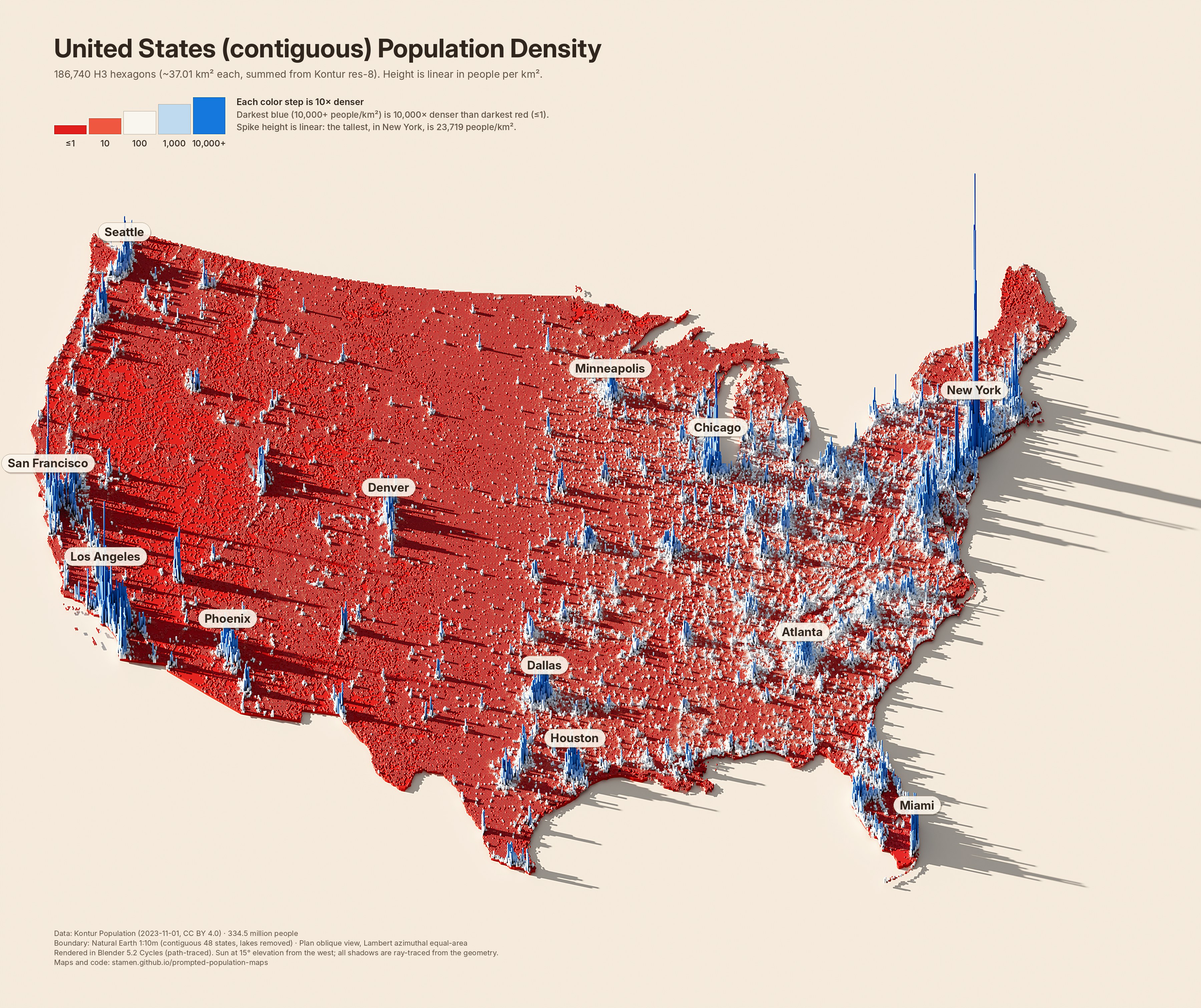
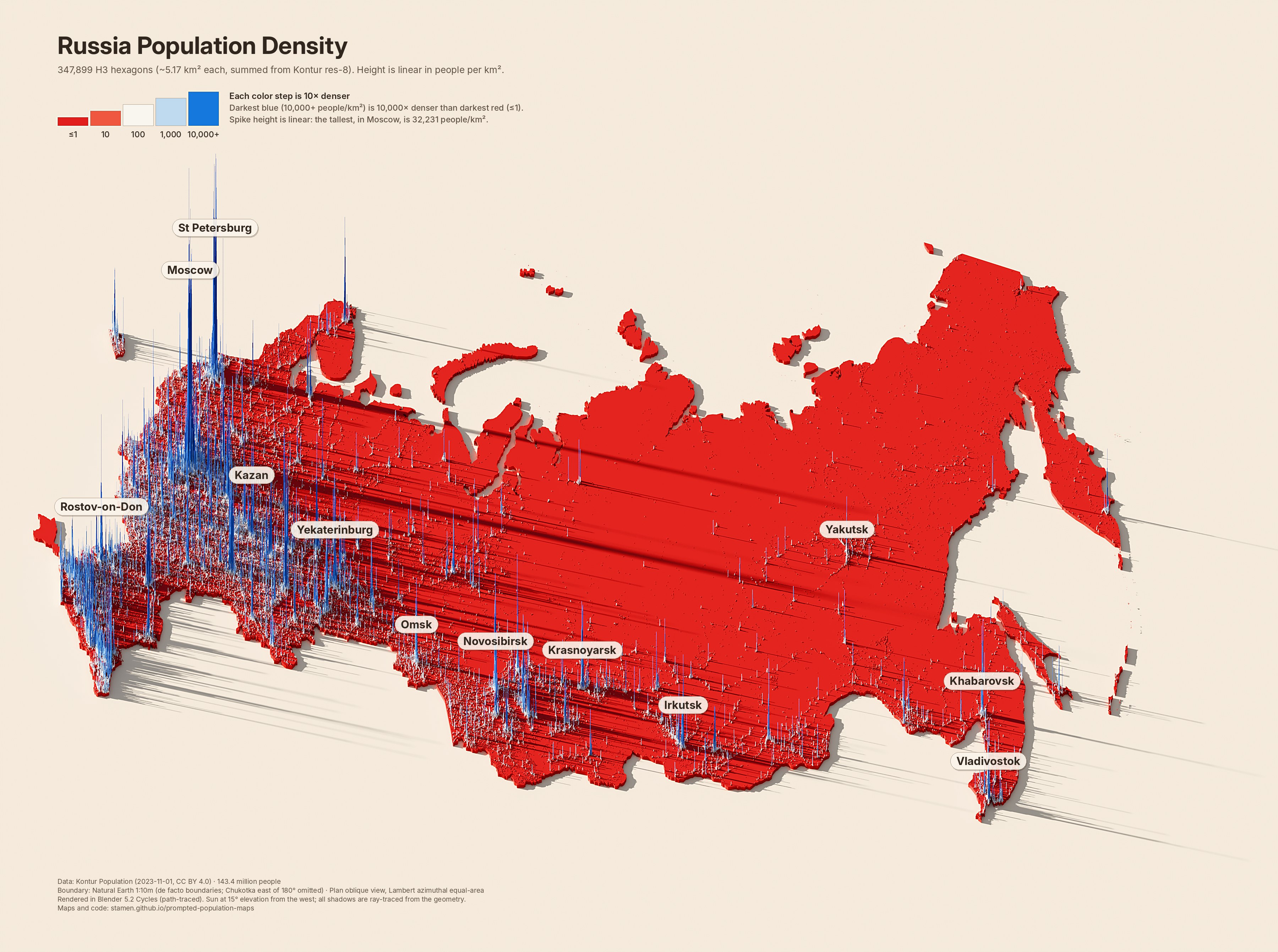
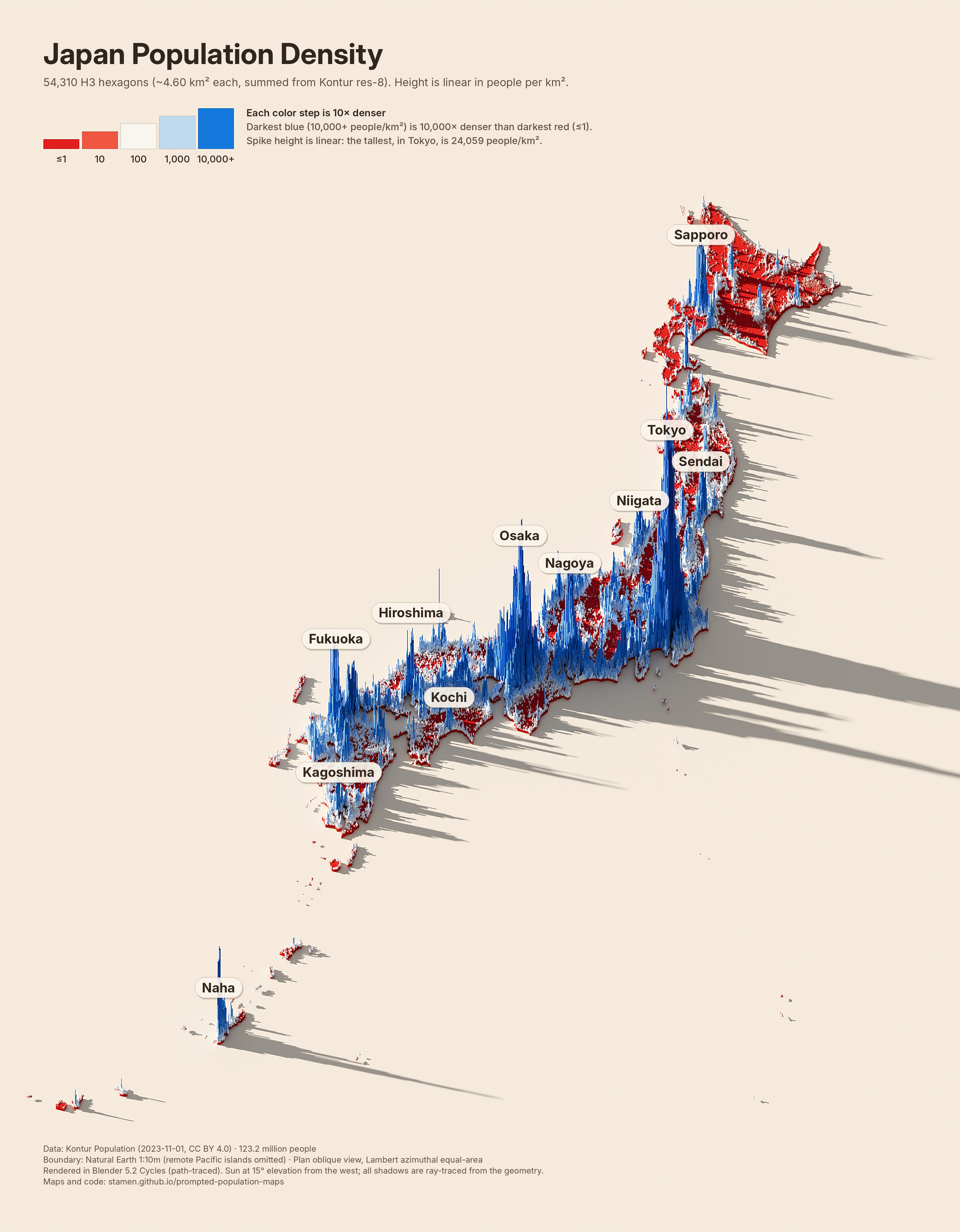
United States (contiguous)334.5 million · 186,740 cells · res 6 (~37.01 km²)Russia143.4 million · 347,899 cells · res 7 (~5.17 km²)Japan123.2 million · 54,310 cells · res 7 (~4.60 km²)Mexico128.6 million · 147,422 cells · res 7 (~6.02 km²)Brazil216.3 million · 599,878 cells · res 7 (~5.60 km²)Australia26.4 million · 218,130 cells · res 7 (~5.91 km²)Egypt112.7 million · 95,697 cells · res 8 (~0.87 km²)
Japan is mostly red and white with blue coastal plains, not blue everywhere: the mountainous interior is nearly empty, which the guessed rural density missed.
Russia's population follows a narrow band along the south of Siberia and the Trans-Siberian corridor, instead of a smooth fade from west to east.
Egypt's people really are confined to the Nile valley and delta, which the vibes version got roughly right, but the real valley is far narrower and the delta far denser.
The contiguous United States, Brazil, and Australia show the texture no guess can supply: highways, rivers, irrigated valleys, and small towns.
The whole United States, at one scale
The contiguous map above leaves out Alaska, Hawaii, and the territories. Here they are, each in its own equal-area projection and moved closer, but not resized: a kilometer is the same length everywhere on this map, which is why Alaska is so large and Guam and American Samoa are specks.
United States340.2 million · 189,820 cells · res 6 (~36.98 km²)
Totals match official figures within about 2%, except Brazil and Egypt, where Kontur's totals (216 and 113 million) follow UN 2023 estimates rather than national counts (Brazil's 2022 census found 203 million; Egypt's statistics agency reported about 105 million in 2023). The Russia map omits the part of Chukotka east of 180°. The US is summed to larger cells (H3 resolution 6, about 36 km²), because at the finer resolution the scene needs more than 14 GB of memory to render. Kontur counts about 604,000 people in Alaska, below the official figure of about 733,000.